

NLP with Bangla: word2vec, generating Bangla text & sentiment analysis (LSTM), ChatBot (RASA NLU)
- Sandipan Dey

- Jan 10, 2021
- 14 min read
Updated: Jan 27, 2021
In this blog, we shall discuss on a few NLP techniques with Bangla language. We shall start with a demonstration on how to train a word2vec model with Bangla wiki corpus with tensorflow and how to visualize the semantic similarity between words using t-SNE. Next, we shall demonstrate how to train a character / word LSTM on selected Tagore’s songs to generate songs like Tagore with keras. Next, we shall create sentiment analysis dataset by crawling the daily astrological prediction pages of a leading Bangla newspaper and manually labeling the sentiment of each of the predictions corresponding to each moon-sign. We shall train an LSTM sentiment a analysis model to predict the sentiment of a moon-sign prediction. Finally, we shall use RASA NLU (natural language understanding) to build a very simple chatbot in Bangla.
Word2vec model with Bangla wiki corpus with tensorflow
Let’s start by importing the required libraries
import collections
import numpy as np
import tensorflow as tf
from matplotlib import pylab
Download the Bangla wikipedia corpus from Kaggle. The first few lines from the corpus are shown below:
id,text,title,url
1528,
“রবীন্দ্রনাথ ঠাকুর”
রবীন্দ্রনাথ ঠাকুর (৭ই মে, ১৮৬১ – ৭ই আগস্ট, ১৯৪১) (২৫ বৈশাখ, ১২৬৮ – ২২ শ্রাবণ, ১৩৪৮ বঙ্গাব্দ) ছিলেন অগ্রণী বাঙালি কবি, ঔপন্যাসিক, সংগীতস্রষ্টা, নাট্যকার, চিত্রকর, ছোটগল্পকার, প্রাবন্ধিক, অভিনেতা, কণ্ঠশিল্পী ও দার্শনিক। তাঁকে বাংলা ভাষার সর্বশ্রেষ্ঠ সাহিত্যিক মনে করা হয়। রবীন্দ্রনাথকে গুরুদেব, কবিগুরু ও বিশ্বকবি অভিধায় ভূষিত করা হয়। রবীন্দ্রনাথের ৫২টি কাব্যগ্রন্থ, ৩৮টি নাটক, ১৩টি উপন্যাস ও ৩৬টি প্রবন্ধ ও অন্যান্য গদ্যসংকলন তাঁর জীবদ্দশায় বা মৃত্যুর অব্যবহিত পরে প্রকাশিত হয়। তাঁর সর্বমোট ৯৫টি ছোটগল্প ও ১৯১৫টি গান যথাক্রমে “”গল্পগুচ্ছ”” ও “”গীতবিতান”” সংকলনের অন্তর্ভুক্ত হয়েছে। রবীন্দ্রনাথের যাবতীয় প্রকাশিত ও গ্রন্থাকারে অপ্রকাশিত রচনা ৩২ খণ্ডে “”রবীন্দ্র রচনাবলী”” নামে প্রকাশিত হয়েছে। রবীন্দ্রনাথের যাবতীয় পত্রসাহিত্য উনিশ খণ্ডে “”চিঠিপত্র”” ও চারটি পৃথক গ্রন্থে প্রকাশিত। এছাড়া তিনি প্রায় দুই হাজার ছবি এঁকেছিলেন। রবীন্দ্রনাথের রচনা বিশ্বের বিভিন্ন ভাষায় অনূদিত হয়েছে। ১৯১৩ সালে “”গীতাঞ্জলি”” কাব্যগ্রন্থের ইংরেজি অনুবাদের জন্য তিনি সাহিত্যে নোবেল পুরস্কার লাভ করেন।রবীন্দ্রনাথ ঠাকুর কলকাতার এক ধনাঢ্য ও সংস্কৃতিবান ব্রাহ্ম পিরালী ব্রাহ্মণ পরিবারে জন্মগ্রহণ করেন। বাল্যকালে প্রথাগত বিদ্যালয়-শিক্ষা তিনি গ্রহণ করেননি; গৃহশিক্ষক রেখে বাড়িতেই তাঁর শিক্ষার ব্যবস্থা করা হয়েছিল। আট বছর বয়সে তিনি কবিতা লেখা শুরু করেন। ১৮৭৪ সালে “”তত্ত্ববোধিনী পত্রিকা””-এ তাঁর “””” কবিতাটি প্রকাশিত হয়। এটিই ছিল তাঁর প্রথম প্রকাশিত রচনা। ১৮৭৮ সালে মাত্র সতেরো বছর বয়সে রবীন্দ্রনাথ প্রথমবার ইংল্যান্ডে যান। ১৮৮৩ সালে মৃণালিনী দেবীর সঙ্গে তাঁর বিবাহ হয়। ১৮৯০ সাল থেকে রবীন্দ্রনাথ পূর্ববঙ্গের শিলাইদহের জমিদারি এস্টেটে বসবাস শুরু করেন। ১৯০১ সালে তিনি পশ্চিমবঙ্গের শান্তিনিকেতনে ব্রহ্মচর্যাশ্রম প্রতিষ্ঠা করেন এবং সেখানেই পাকাপাকিভাবে বসবাস শুরু করেন। ১৯০২ সালে তাঁর পত্নীবিয়োগ হয়। ১৯০৫ সালে তিনি বঙ্গভঙ্গ-বিরোধী আন্দোলনে জড়িয়ে পড়েন। ১৯১৫ সালে ব্রিটিশ সরকার তাঁকে নাইট উপাধিতে ভূষিত করেন। কিন্তু ১৯১৯ সালে জালিয়ানওয়ালাবাগ হত্যাকাণ্ডের প্রতিবাদে তিনি সেই উপাধি ত্যাগ করেন। ১৯২১ সালে গ্রামোন্নয়নের জন্য তিনি শ্রীনিকেতন নামে একটি সংস্থা প্রতিষ্ঠা করেন। ১৯২৩ সালে আনুষ্ঠানিকভাবে বিশ্বভারতী প্রতিষ্ঠিত হয়। দীর্ঘজীবনে তিনি বহুবার বিদেশ ভ্রমণ করেন এবং সমগ্র বিশ্বে বিশ্বভ্রাতৃত্বের বাণী প্রচার করেন। ১৯৪১ সালে দীর্ঘ রোগভোগের পর কলকাতার পৈত্রিক বাসভবনেই তাঁর মৃত্যু হয়।রবীন্দ্রনাথের কাব্যসাহিত্যের বৈশিষ্ট্য ভাবগভীরতা, গীতিধর্মিতা চিত্ররূপময়তা, অধ্যাত্মচেতনা, ঐতিহ্যপ্রীতি, প্রকৃতিপ্রেম, মানবপ্রেম, স্বদেশপ্রেম, বিশ্বপ্রেম, রোম্যান্টিক সৌন্দর্যচেতনা, ভাব, ভাষা, ছন্দ ও আঙ্গিকের বৈচিত্র্য, বাস্তবচেতনা ও প্রগতিচেতনা। রবীন্দ্রনাথের গদ্যভাষাও কাব্যিক। ভারতের ধ্রুপদি ও লৌকিক সংস্কৃতি এবং পাশ্চাত্য বিজ্ঞানচেতনা ও শিল্পদর্শন তাঁর রচনায় গভীর প্রভাব বিস্তার করেছিল। কথাসাহিত্য ও প্রবন্ধের মাধ্যমে তিনি সমাজ, রাজনীতি ও রাষ্ট্রনীতি সম্পর্কে নিজ মতামত প্রকাশ করেছিলেন। সমাজকল্যাণের উপায় হিসেবে তিনি গ্রামোন্নয়ন ও গ্রামের দরিদ্র মানুষ কে শিক্ষিত করে তোলার পক্ষে মতপ্রকাশ করেন। এর পাশাপাশি সামাজিক ভেদাভেদ, অস্পৃশ্যতা, ধর্মীয় গোঁড়ামি ও ধর্মান্ধতার বিরুদ্ধেও তিনি তীব্র প্রতিবাদ জানিয়েছিলেন। রবীন্দ্রনাথের দর্শনচেতনায় ঈশ্বরের মূল হিসেবে মানব সংসারকেই নির্দিষ্ট করা হয়েছে; রবীন্দ্রনাথ দেববিগ্রহের পরিবর্তে কর্মী অর্থাৎ মানুষ ঈশ্বরের পূজার কথা বলেছিলেন। সংগীত ও নৃত্যকে তিনি শিক্ষার অপরিহার্য অঙ্গ মনে করতেন। রবীন্দ্রনাথের গান তাঁর অন্যতম শ্রেষ্ঠ কীর্তি। তাঁর রচিত “”আমার সোনার বাংলা”” ও “”জনগণমন-অধিনায়ক জয় হে”” গানদুটি যথাক্রমে গণপ্রজাতন্ত্রী বাংলাদেশ ও ভারতীয় প্রজাতন্ত্রের জাতীয় সংগীত।
জীবন.
প্রথম জীবন (১৮৬১–১৯০১).
শৈশব ও কৈশোর (১৮৬১ – ১৮৭৮).
রবীন্দ্রনাথ ঠাকুর কলকাতার জোড়াসাঁকো ঠাকুরবাড়িতে জন্মগ্রহণ করেছিলেন। তাঁর পিতা ছিলেন ব্রাহ্ম ধর্মগুরু দেবেন্দ্রনাথ ঠাকুর (১৮১৭–১৯০৫) এবং মাতা ছিলেন সারদাসুন্দরী দেবী (১৮২৬–১৮৭৫)। রবীন্দ্রনাথ ছিলেন পিতামাতার চতুর্দশ সন্তান। জোড়াসাঁকোর ঠাকুর পরিবার ছিল ব্রাহ্ম আদিধর্ম মতবাদের প্রবক্তা। রবীন্দ্রনাথের পূর্ব পুরুষেরা খুলনা জেলার রূপসা উপজেলা পিঠাভোগে বাস করতেন। ১৮৭৫ সালে মাত্র চোদ্দ বছর বয়সে রবীন্দ্রনাথের মাতৃবিয়োগ ঘটে। পিতা দেবেন্দ্রনাথ দেশভ্রমণের নেশায় বছরের অধিকাংশ সময় কলকাতার বাইরে অতিবাহিত করতেন। তাই ধনাঢ্য পরিবারের সন্তান হয়েও রবীন্দ্রনাথের ছেলেবেলা কেটেছিল ভৃত্যদের অনুশাসনে। শৈশবে রবীন্দ্রনাথ কলকাতার ওরিয়েন্টাল সেমিনারি, নর্ম্যাল স্কুল, বেঙ্গল অ্যাকাডেমি এবং সেন্ট জেভিয়ার্স কলেজিয়েট স্কুলে কিছুদিন করে পড়াশোনা করেছিলেন। কিন্তু বিদ্যালয়-শিক্ষায় অনাগ্রহী হওয়ায় বাড়িতেই গৃহশিক্ষক রেখে তাঁর শিক্ষার ব্যবস্থা করা হয়েছিল। ছেলেবেলায় জোড়াসাঁকোর বাড়িতে অথবা বোলপুর ও পানিহাটির বাগানবাড়িতে প্রাকৃতিক পরিবেশের মধ্যে ঘুরে বেড়াতে বেশি স্বচ্ছন্দবোধ করতেন রবীন্দ্রনাথ।১৮৭৩ সালে এগারো বছর বয়সে রবীন্দ্রনাথের উপনয়ন অনুষ্ঠিত হয়েছিল। এরপর তিনি কয়েক মাসের জন্য পিতার সঙ্গে দেশভ্রমণে বের হন। প্রথমে তাঁরা আসেন শান্তিনিকেতনে। এরপর পাঞ্জাবের অমৃতসরে কিছুকাল কাটিয়ে শিখদের উপাসনা পদ্ধতি পরিদর্শন করেন। শেষে পুত্রকে নিয়ে দেবেন্দ্রনাথ যান পাঞ্জাবেরই (অধুনা ভারতের হিমাচল প্রদেশ রাজ্যে অবস্থিত) ডালহৌসি শৈলশহরের নিকট বক্রোটায়। এখানকার বক্রোটা বাংলোয় বসে রবীন্দ্রনাথ পিতার কাছ থেকে সংস্কৃত ব্যাকরণ, ইংরেজি, জ্যোতির্বিজ্ঞান, সাধারণ বিজ্ঞান ও ইতিহাসের নিয়মিত পাঠ নিতে শুরু করেন। দেবেন্দ্রনাথ তাঁকে বিশিষ্ট ব্যক্তিবর্গের জীবনী, কালিদাস রচিত ধ্রুপদি সংস্কৃত কাব্য ও নাটক এবং উপনিষদ্ পাঠেও উৎসাহিত করতেন। ১৮৭৭ সালে “”ভারতী”” পত্রিকায় তরুণ রবীন্দ্রনাথের কয়েকটি গুরুত্বপূর্ণ রচনা প্রকাশিত হয়। এগুলি হল মাইকেল মধুসূদনের “”””, “”ভানুসিংহ ঠাকুরের পদাবলী”” এবং “””” ও “””” নামে দুটি গল্প। এর মধ্যে “”ভানুসিংহ ঠাকুরের পদাবলী”” বিশেষভাবে উল্লেখযোগ্য। এই কবিতাগুলি রাধা-কৃষ্ণ বিষয়ক পদাবলির অনুকরণে “”ভানুসিংহ”” ভণিতায় রচিত। রবীন্দ্রনাথের “”ভিখারিণী”” গল্পটি (১৮৭৭) বাংলা সাহিত্যের প্রথম ছোটগল্প। ১৮৭৮ সালে প্রকাশিত হয় রবীন্দ্রনাথের প্রথম কাব্যগ্রন্থ তথা প্রথম মুদ্রিত গ্রন্থ “”কবিকাহিনী””। এছাড়া এই পর্বে তিনি রচনা করেছিলেন “””” (১৮৮২) কাব্যগ্রন্থটি। রবীন্দ্রনাথের বিখ্যাত কবিতা “””” এই কাব্যগ্রন্থের অন্তর্গত।
যৌবন (১৮৭৮-১৯০১).
১৮৭৮ সালে ব্যারিস্টারি পড়ার উদ্দেশ্যে ইংল্যান্ডে যান রবীন্দ্রনাথ। প্রথমে তিনি ব্রাইটনের একটি পাবলিক স্কুলে ভর্তি হয়েছিলেন। ১৮৭৯ সালে ইউনিভার্সিটি কলেজ লন্ডনে আইনবিদ্যা নিয়ে পড়াশোনা শুরু করেন। কিন্তু সাহিত্যচর্চার আকর্ষণে সেই পড়াশোনা তিনি সমাপ্ত করতে পারেননি। ইংল্যান্ডে থাকাকালীন শেকসপিয়র ও অন্যান্য ইংরেজ সাহিত্যিকদের রচনার সঙ্গে রবীন্দ্রনাথের পরিচয় ঘটে। এই সময় তিনি বিশেষ মনোযোগ সহকারে পাঠ করেন “”রিলিজিও মেদিচি””, “”কোরিওলেনাস”” এবং “”অ্যান্টনি অ্যান্ড ক্লিওপেট্রা””। এই সময় তাঁর ইংল্যান্ডবাসের অভিজ্ঞতার কথা “”ভারতী”” পত্রিকায় পত্রাকারে পাঠাতেন রবীন্দ্রনাথ। উক্ত পত্রিকায় এই লেখাগুলি জ্যেষ্ঠভ্রাতা দ্বিজেন্দ্রনাথ ঠাকুরের সমালোচনাসহ প্রকাশিত হত “””” নামে। ১৮৮১ সালে সেই পত্রাবলি “””” নামে গ্রন্থাকারে ছাপা হয়। এটিই ছিল রবীন্দ্রনাথের প্রথম গদ্যগ্রন্থ তথা প্রথম চলিত ভাষায় লেখা গ্রন্থ। অবশেষে ১৮৮০ সালে প্রায় দেড় বছর ইংল্যান্ডে কাটিয়ে কোনো ডিগ্রি না নিয়ে এবং ব্যারিস্টারি পড়া শুরু না করেই তিনি দেশে ফিরে আসেন।১৮৮৩ সালের ৯ ডিসেম্বর (২৪ অগ্রহায়ণ, ১২৯০ বঙ্গাব্দ) ঠাকুরবাড়ির অধস্তন কর্মচারী বেণীমাধব রায়চৌধুরীর কন্যা ভবতারিণীর সঙ্গে রবীন্দ্রনাথের বিবাহ সম্পন্ন হয়। বিবাহিত জীবনে ভবতারিণীর নামকরণ হয়েছিল মৃণালিনী দেবী (১৮৭৩–১৯০২ )। রবীন্দ্রনাথ ও মৃণালিনীর সন্তান ছিলেন পাঁচ জন: মাধুরীলতা (১৮৮৬–১৯১৮), রথীন্দ্রনাথ (১৮৮৮–১৯৬১), রেণুকা (১৮৯১–১৯০৩), মীরা (১৮৯৪–১৯৬৯) এবং শমীন্দ্রনাথ (১৮৯৬–১৯০৭)। এঁদের মধ্যে অতি অল্প বয়সেই রেণুকা ও শমীন্দ্রনাথের মৃত্যু ঘটে।১৮৯১ সাল থেকে পিতার আদেশে নদিয়া (নদিয়ার উক্ত অংশটি অধুনা বাংলাদেশের কুষ্টিয়া জেলা), পাবনা ও রাজশাহী জেলা এবং উড়িষ্যার জমিদারিগুলির তদারকি শুরু করেন রবীন্দ্রনাথ। কুষ্টিয়ার শিলাইদহের কুঠিবাড়িতে রবীন্দ্রনাথ দীর্ঘ সময় অতিবাহিত করেছিলেন। জমিদার রবীন্দ্রনাথ শিলাইদহে “”পদ্মা”” নামে একটি বিলাসবহুল পারিবারিক বজরায় চড়ে প্রজাবর্গের কাছে খাজনা আদায় ও আশীর্বাদ প্রার্থনা করতে যেতেন। গ্রামবাসীরাও তাঁর সম্মানে ভোজসভার আয়োজন করত।১৮৯০ সালে রবীন্দ্রনাথের অপর বিখ্যাত কাব্যগ্রন্থ “””” প্রকাশিত হয়। কুড়ি থেকে ত্রিশ বছর বয়সের মধ্যে তাঁর আরও কয়েকটি উল্লেখযোগ্য কাব্যগ্রন্থ ও গীতিসংকলন প্রকাশিত হয়েছিল। এগুলি হলো “”””, “”””, “”রবিচ্ছায়া””, “””” ইত্যাদি। ১৮৯১ থেকে ১৮৯৫ সাল পর্যন্ত নিজের সম্পাদিত “”সাধনা”” পত্রিকায় রবীন্দ্রনাথের বেশ কিছু উৎকৃষ্ট রচনা প্রকাশিত হয়। তাঁর সাহিত্যজীবনের এই পর্যায়টি তাই “”সাধনা পর্যায়”” নামে পরিচিত। রবীন্দ্রনাথের “”গল্পগুচ্ছ”” গ্রন্থের প্রথম চুরাশিটি গল্পের অর্ধেকই এই পর্যায়ের রচনা। এই ছোটগল্পগুলিতে তিনি বাংলার গ্রামীণ জনজীবনের এক আবেগময় ও শ্লেষাত্মক চিত্র এঁকেছিলেন।Preprocess the csv files with the following code using regular expressions (to get rid of punctuations). Remember we need to decode to utf-8 first, since we have unicode input files.
from glob import glob
import re
words = []
for f in glob('bangla/wiki/*.csv'):
 words += re.sub('[\r\n—?,;।!‘"’\.:\(\)\[\]…0-9]', ' ', \
          open(f, 'rb').read().decode('utf8').strip()).split(' ')
words = list(filter(lambda x: not x in ['', '-'], words))
print(len(words))
# 13964346
words[:25]
#['রবীন্দ্রনাথ',
# 'ঠাকুর',
# 'রবীন্দ্রনাথ',
# 'ঠাকুর',
# '৭ই',
# 'মে',
# '১৮৬১',
# '৭ই',
# 'আগস্ট',
# '১৯৪১',
# '২৫',
# 'বৈশাখ',
# '১২৬৮',
# '২২',
# 'শ্রাবণ',
# '১৩৪৮',
# 'বঙ্গাব্দ',
# 'ছিলেন',
# 'অগ্রণী',
# 'বাঙালি',
# 'কবি',
# 'ঔপন্যাসিক',
# 'সংগীতস্রষ্টা',
# 'নাট্যকার',
# 'চিত্রকর']
Create indices for unique words in the dataset.
vocabulary_size = 25000
def build_dataset(words):
  count = [['UNK', -1]]
  count.extend(collections.Counter(words) \
              .most_common(vocabulary_size - 1))
  dictionary = dict()
  for word, _ in count:
    dictionary[word] = len(dictionary)
  data = list()
  unk_count = 0
  for word in words:
    if word in dictionary:
      index = dictionary[word]
    else:
      index = 0  # dictionary['UNK']
      unk_count = unk_count + 1
    data.append(index)
  count[0][1] = unk_count
  reverse_dictionary = dict(zip(dictionary.values(), \
                                dictionary.keys()))
  return data, count, dictionary, reverse_dictionary

data, count, dictionary, reverse_dictionary = build_dataset(words)
print('Most common words (+UNK)', count[:5])
# Most common words (+UNK) [['UNK', 1961151], ('এবং', 196916),
# ('ও', 180042), ('হয়', 160533), ('করে', 131206)]
print('Sample data', data[:10])
#Sample data [1733, 1868, 1733, 1868, 5769, 287, 6855, 5769, 400, 2570]
del words  # Hint to reduce memory.
Generate batches to be trained with the word2vec skip-gram model.
The target label should be at the center of the buffer each time. That is, given a focus word, our goal will be to learn the most probable context words.
The input and the target vector will depend on num_skips and skip_window.
data_index = 0
def generate_batch(batch_size, num_skips, skip_window):
  global data_index
  assert batch_size % num_skips == 0
  assert num_skips <= 2 * skip_window
  batch = np.ndarray(shape=(batch_size), dtype=np.int32)
  labels = np.ndarray(shape=(batch_size, 1), dtype=np.int32)
  span = 2 * skip_window + 1 # [ skip_window target skip_window ]
  buffer = collections.deque(maxlen=span)
  for _ in range(span):
    buffer.append(data[data_index])
    data_index = (data_index + 1) % len(data)
  for i in range(batch_size // num_skips):
    target = skip_window  #
    targets_to_avoid = [ skip_window ]
    for j in range(num_skips):
      while target in targets_to_avoid:
        target = random.randint(0, span - 1)
      targets_to_avoid.append(target)
      batch[i * num_skips + j] = buffer[skip_window]
      labels[i * num_skips + j, 0] = buffer[target]
    buffer.append(data[data_index])
    data_index = (data_index + 1) % len(data)
  return batch, labels

print('data:', [reverse_dictionary[di] for di in data[:8]])
# data: ['রবীন্দ্রনাথ', 'ঠাকুর', 'রবীন্দ্রনাথ', 'ঠাকুর', '৭ই', 'মে',
# '১৮৬১', '৭ই']
for num_skips, skip_window in [(2, 1), (4, 2)]:
    data_index = 0
    batch, labels = generate_batch(batch_size=8, num_skips=num_skips, \
                                   skip_window=skip_window)
    print('\nwith num_skips = %d and skip_window = %d:' %
                                    (num_skips, skip_window))
    print('batch:', [reverse_dictionary[bi] for bi in batch])
    print('labels:', [reverse_dictionary[li] for li in \
                                      labels.reshape(8)])
    # data: ['রবীন্দ্রনাথ', 'ঠাকুর', 'রবীন্দ্রনাথ', 'ঠাকুর', '৭ই', 'মে',
    # '১৮৬১', '৭ই']
    # with num_skips = 2 and skip_window = 1:
    # batch: ['ঠাকুর', 'ঠাকুর', 'রবীন্দ্রনাথ', 'রবীন্দ্রনাথ', 'ঠাকুর', 'ঠাকুর',
    # '৭ই', '৭ই']
    # labels: ['রবীন্দ্রনাথ', 'রবীন্দ্রনাথ', 'ঠাকুর', 'ঠাকুর', '৭ই', 'রবীন্দ্রনাথ',
    # 'ঠাকুর', 'মে']
    # with num_skips = 4 and skip_window = 2:
    # batch: ['রবীন্দ্রনাথ', 'রবীন্দ্রনাথ', 'রবীন্দ্রনাথ', 'রবীন্দ্রনাথ', 'ঠাকুর',
    # 'ঠাকুর', 'ঠাকুর', 'ঠাকুর']
    # labels: ['রবীন্দ্রনাথ', '৭ই', 'ঠাকুর', 'ঠাকুর', 'মে', 'ঠাকুর',
    # 'রবীন্দ্রনাথ', '৭ই']
Pick a random validation set to sample nearest neighbors.
Limit the validation samples to the words that have a low numeric ID, which by construction are also the most frequent.
Look up embeddings for inputs and compute the softmax loss, using a sample of the negative labels each time (this is known as negative sampling, which is used to make the computation efficient, since the number of labels are often too high).
The optimizer will optimize the softmax_weights and the embeddings. This is because the embeddings are defined as a variable quantity and the optimizer’s `minimize` method will by default modify all variable quantities that contribute to the tensor it is passed.
Compute the similarity between minibatch examples and all embeddings.
 batch_size = 128
 embedding_size = 128 # Dimension of the embedding vector.
 skip_window = 1 # How many words to consider left and right.
 num_skips = 2 # #times to reuse an input to generate a label.
 valid_size = 16 # Random set of words to evaluate similarity on.
 valid_window = 100 # Only pick dev samples in the head of the
                    # distribution.
 valid_examples = np.array(random.sample(range(valid_window),
                                         valid_size))
 num_sampled = 64 # Number of negative examples to sample.
 graph = tf.Graph()

 with graph.as_default(), tf.device('/cpu:0'):
 # Input data.
   train_dataset = tf.placeholder(tf.int32, shape=[batch_size])
   train_labels = tf.placeholder(tf.int32, shape=[batch_size, 1])
   valid_dataset = tf.constant(valid_examples, dtype=tf.int32)
 # Variables.
   embeddings = tf.Variable( \
     tf.random_uniform([vocabulary_size, embedding_size], -1.0, 1.0))
   softmax_weights = tf.Variable( \
     tf.truncated_normal([vocabulary_size, embedding_size], \
                          stddev=1.0 / math.sqrt(embedding_size)))
   softmax_biases = tf.Variable(tf.zeros([vocabulary_size]))
 # Model.
   embed = tf.nn.embedding_lookup(embeddings, train_dataset)
   loss = tf.reduce_mean( \
                          tf.nn.sampled_softmax_loss(weights=softmax_weights, \
                          biases=softmax_biases, inputs=embed, \
                          labels=train_labels, \
                          num_sampled=num_sampled, \
                          num_classes=vocabulary_size))
 # Optimizer.
 optimizer = tf.train.AdagradOptimizer(1.0).minimize(loss)
 # use the cosine distance:
 norm = tf.sqrt(tf.reduce_sum(tf.square(embeddings), 1, keepdims=True))
   normalized_embeddings = embeddings / norm
   valid_embeddings = tf.nn.embedding_lookup(normalized_embeddings, \
                                             valid_dataset)
   similarity = tf.matmul(valid_embeddings, \
                          tf.transpose(normalized_embeddings))
Train the word2vec model with the batches constructed, for 100k steps.
num_steps = 100001
with tf.Session(graph=graph) as session:
  tf.global_variables_initializer().run()
  print('Initialized')
  average_loss = 0
  for step in range(num_steps):
    batch_data, batch_labels = generate_batch(
      batch_size, num_skips, skip_window)
    feed_dict = {train_dataset : batch_data, \
                 train_labels : batch_labels}
    _, l = session.run([optimizer, loss], feed_dict=feed_dict)
    average_loss += l
    if step % 2000 == 0:
      if step > 0:
        average_loss = average_loss / 2000
      # The average loss is an estimate of the loss over the last
      # 2000 batches.
      print('Average loss at step %d: %f' % (step, average_loss))
      average_loss = 0
      # note that this is expensive (~20% slowdown if computed every
      # 500 steps)
    if step % 10000 == 0:
      sim = similarity.eval()
      for i in range(valid_size):
        valid_word = reverse_dictionary[valid_examples[i]]
        top_k = 8 # number of nearest neighbors
        nearest = (-sim[i, :]).argsort()[1:top_k+1]
        log = 'Nearest to %s:' % valid_word
        for k in range(top_k):
          close_word = reverse_dictionary[nearest[k]]
          log = '%s %s,' % (log, close_word)
        print(log)
  final_embeddings = normalized_embeddings.eval()
The following shows how the loss function decreases with the increase in training steps.
During the training process, the words that become semantically near come closer in the embedding space.
Use t-SNE plot to map the following words from 128-dimensional embedding space to 2 dimensional manifold and visualize.
words = ['রাজা', 'রাণী', 'ভারত','বাংলাদেশ','দিল্লী','কলকাতা','ঢাকা',
 'পুরুষ','নারী','দুঃখ','লেখক','কবি','কবিতা','দেশ',
 'বিদেশ','লাভ','মানুষ', 'এবং', 'ও', 'গান', 'সঙ্গীত', 'বাংলা',
 'ইংরেজি', 'ভাষা', 'কাজ', 'অনেক', 'জেলার', 'বাংলাদেশের',
 'এক', 'দুই', 'তিন', 'চার', 'পাঁচ', 'দশ', '১', '৫', '২০',
 'নবম', 'ভাষার', '১২', 'হিসাবে', 'যদি', 'পান', 'শহরের', 'দল',
 'যদিও', 'বলেন', 'রান', 'করেছে', 'করে', 'এই', 'করেন', 'তিনি',
 'একটি', 'থেকে', 'করা', 'সালে', 'এর', 'যেমন', 'সব',  'তার',
 'খেলা',  'অংশ', 'উপর', 'পরে', 'ফলে',  'ভূমিকা', 'গঠন',
 'তা', 'দেন', 'জীবন', 'যেখানে', 'খান', 'এতে',  'ঘটে', 'আগে',
 'ধরনের', 'নেন', 'করতেন', 'তাকে', 'আর', 'যার', 'দেখা',
 'বছরের', 'উপজেলা', 'থাকেন', 'রাজনৈতিক', 'মূলত', 'এমন',
 'কিলোমিটার', 'পরিচালনা', '২০১১', 'তারা', 'তিনি', 'যিনি', 'আমি',
 'তুমি', 'আপনি', 'লেখিকা', 'সুখ', 'বেদনা', 'মাস', 'নীল', 'লাল',
 'সবুজ', 'সাদা', 'আছে', 'নেই', 'ছুটি', 'ঠাকুর',
 'দান', 'মণি', 'করুণা', 'মাইল', 'হিন্দু', 'মুসলমান','কথা', 'বলা',
 'সেখানে', 'তখন', 'বাইরে', 'ভিতরে', 'ভগবান' ]
indices = []
for word in words:
 #print(word, dictionary[word])
 indices.append(dictionary[word])
two_d_embeddings = tsne.fit_transform(final_embeddings[indices, :])
plot(two_d_embeddings, words)
The following figure shows how the words similar in meaning are mapped to embedding vectors that are close to each other.

Also, note that arithmetic property of the word embeddings: e.g., the words ‘রাজা’ and ‘রাণী’ are approximately along the same distance and direction as the words ‘লেখক’ and ‘লেখিকা’, reflecting the fact that the nature of the semantic relatedness in terms of gender is same.
The following animation shows how the embedding is learnt to preserve the semantic similarity in the 2D-manifold more and more as training proceeds.\

Generating song-like texts with LSTM from Tagore’s Bangla songs
Text generation with Character LSTM
Let’s import the required libraries first.
from tensorflow.keras.callbacks import LambdaCallback
from tensorflow.keras.models import Sequential
from tensorflow.keras.layers import Dense
from tensorflow.keras.layers import LSTM
from tensorflow.keras.optimizers import RMSprop, Adam
import io, re
Read the input file, containing few selected songs of Tagore in Bangla.
raw_text = open('rabindrasangeet.txt','rb').read().decode('utf8')
print(raw_text[0:1000])
পূজা
অগ্নিবীণা বাজাও তুমি
অগ্নিবীণা বাজাও তুমি কেমন ক’রে !
আকাশ কাঁপে তারার আলোর গানের ঘোরে ।।
তেমনি ক’রে আপন হাতে ছুঁলে আমার বেদনাতে,
নূতন সৃষ্টি জাগল বুঝি জীবন-‘পরে ।।
বাজে ব’লেই বাজাও তুমি সেই গরবে,
ওগো প্রভু, আমার প্রাণে সকল সবে ।
বিষম তোমার বহ্নিঘাতে বারে বারে আমার রাতে
জ্বালিয়ে দিলে নূতন তারা ব্যথায় ভ’রে ।।
অচেনাকে ভয় কী
অচেনাকে ভয় কী আমার ওরে?
অচেনাকেই চিনে চিনে উঠবে জীবন ভরে ।।
জানি জানি আমার চেনা কোনো কালেই ফুরাবে না,
চিহ্নহারা পথে আমায় টানবে অচিন ডোরে ।।
ছিল আমার মা অচেনা, নিল আমায় কোলে ।
সকল প্রেমই অচেনা গো, তাই তো হৃদয় দোলে ।
অচেনা এই ভুবন-মাঝে কত সুরেই হৃদয় বাজে-
অচেনা এই জীবন আমার, বেড়াই তারি ঘোরে ।।অন্তর মম
অন্তর মম বিকশিত করো অন্তরতর হে-
নির্মল করো, উজ্জ্বল করো, সুন্দর করো হে ।।
জাগ্রত করো, উদ্যত করো, নির্ভয় করো হে ।।
মঙ্গল করো, নিরলস নিঃসংশয় করো হে ।।
যুক্ত করো হে সবার সঙ্গে, মুক্ত করো হে বন্ধ ।
সঞ্চার করো সকল কর্মে শান্ত তোমার ছন্দ ।
চরণপদ্মে মম চিত নিস্পন্দিত করো হে ।
নন্দিত করো, নন্দিত করো, নন্দিত করো হে ।।
অন্তরে জাগিছ অন্তর্যামী
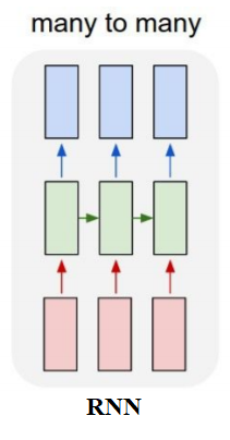
অন্তরে জাগিছ অন্তর্যামী ।Here we shall be using a many-to-many RNN as shown in the next figure.
Pre-process the text and create character indices to be used as the input in the model.
processed_text = raw_text.lower()
print('corpus length:', len(processed_text))
# corpus length: 207117
chars = sorted(list(set(processed_text)))
print('total chars:', len(chars))
# total chars: 89
char_indices = dict((c, i) for i, c in enumerate(chars))
indices_char = dict((i, c) for i, c in enumerate(chars))
Cut the text in semi-redundant sequences of maxlen characters.
def is_conjunction(c):
 h = ord(c) # print(hex(ord(c)))
 return (h >= 0x980 and h = 0x9bc and h = 0x9f2)

maxlen = 40
step = 2
sentences = []
next_chars = []
i = 0
while i < len(processed_text) - maxlen:
 if is_conjunction(processed_text[i]):
   i += 1
   continue
 sentences.append(processed_text[i: i + maxlen])
 next_chars.append(processed_text[i + maxlen])
 i += step
 print('nb sequences:', len(sentences))
 # nb sequences: 89334
Create one-hot-encodings.
x = np.zeros((len(sentences), maxlen, len(chars)), dtype=np.bool)
y = np.zeros((len(sentences), len(chars)), dtype=np.bool)
for i, sentence in enumerate(sentences):
 for t, char in enumerate(sentence):
 x[i, t, char_indices[char]] = 1
 y[i, char_indices[next_chars[i]]] = 1
Build a model, a single LSTM.
model = Sequential()
model.add(LSTM(256, input_shape=(maxlen, len(chars))))
model.add(Dense(128, activation='relu'))
model.add(Dense(len(chars), activation='softmax'))
optimizer = Adam(lr=0.01) #RMSprop(lr=0.01)
model.compile(loss='categorical_crossentropy', optimizer=optimizer)
The following figure how the model architecture looks like:
Print the model summary.
model.summary()

Model: "sequential"
_________________________________________________________________
Layer (type)                 Output Shape              Param #
=================================================================
lstm (LSTM)                  (None, 256)               354304
_________________________________________________________________
dense (Dense)                (None, 128)               32896
_________________________________________________________________
dense_1 (Dense)              (None, 89)                11481
=================================================================
Total params: 398,681 Trainable params: 398,681 Non-trainable params: 0
_________________________________________________________________
Use the following helper function to sample an index from a probability array.
def sample(preds, temperature=1.0):
 preds = np.asarray(preds).astype('float64')
 preds = np.log(preds) / temperature
 exp_preds = np.exp(preds)
 preds = exp_preds / np.sum(exp_preds)
 probas = np.random.multinomial(1, preds, 1)
 return np.argmax(probas)
Fit the model and register a callback to print the text generated by the model at the end of each epoch.
print_callback = LambdaCallback(on_epoch_end=on_epoch_end)
model.fit(x, y, batch_size=128, epochs=60, callbacks=[print_callback])
The following animation shows how the model generates song-like texts with given seed texts, for different values of the temperature parameter.
Text Generation with Word LSTM
Pre-process the input text, split by punctuation characters and create word indices to be used as the input in the model.
processed_text = raw_text.lower()
from string import punctuation
r = re.compile(r'[\s{}]+'.format(re.escape(punctuation)))
words = r.split(processed_text)
print(len(words))
words[:16]
39481
# ['পূজা',
# 'অগ্নিবীণা',
# 'বাজাও',
# 'তুমি',
# 'অগ্নিবীণা',
# 'বাজাও',
# 'তুমি',
# 'কেমন',
# 'ক’রে',
# 'আকাশ',
# 'কাঁপে',
# 'তারার',
# 'আলোর',
# 'গানের',
# 'ঘোরে',
# '।।']

unique_words = np.unique(words)
unique_word_index = dict((c, i) for i, c in enumerate(unique_words))
index_unique_word = dict((i, c) for i, c in enumerate(unique_words))
Create a word-window of length 5 to predict the next word.
WORD_LENGTH = 5
prev_words = []
next_words = []
for i in range(len(words) - WORD_LENGTH):
    prev_words.append(words[i:i + WORD_LENGTH])
    next_words.append(words[i + WORD_LENGTH])
print(prev_words[1])
# ['অগ্নিবীণা', 'বাজাও', 'তুমি', 'অগ্নিবীণা', 'বাজাও']
print(next_words[1])
# তুমি
print(len(unique_words))
# 7847
Create OHE for input and output words as done for character-RNN. Fit the model on the pre-rpocessed data.
print_callback = LambdaCallback(on_epoch_end=on_epoch_end)
model.fit(X, Y,
          batch_size=128,
          epochs=60,
          callbacks=[print_callback])
The following animation shows the song -like text generated by the word-LSTM at the end of an epoc.

Bangla Sentiment Analysis using LSTM with Daily Astrological Prediction Dataset
Let's first create sentiment analysis dataset by crawling the daily horoscope prediction (রাশিফল) page of the online edition of আনন্দবাজার পত্রিকা (e.g., for the year 2013), a leading Bangla newspaper and then manually labeling the sentiment of each of the predictions corresponding to each moon-sign.
Read the csv dataset, the first few lines look like the following.
df = pd.read_csv('horo_2013_labeled.csv')
pd.set_option('display.max_colwidth', 135)
df.head(20)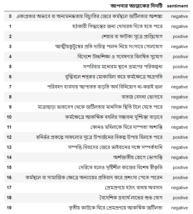
Transform each text in texts in a sequence of integers.
tokenizer = Tokenizer(num_words=2000, split=' ')
tokenizer.fit_on_texts(df['আপনার আজকের দিনটি'].values)
X = tokenizer.texts_to_sequences(df['আপনার আজকের দিনটি'].values)
X = pad_sequences(X)
X
#array([[ 0, 0, 0, ..., 26, 375, 3],
# [ 0, 0, 0, ..., 54, 8, 1],
# [ 0, 0, 0, ..., 108, 42, 43],
# ...,
# [ 0, 0, 0, ..., 1336, 302, 82],
# [ 0, 0, 0, ..., 1337, 489, 218],
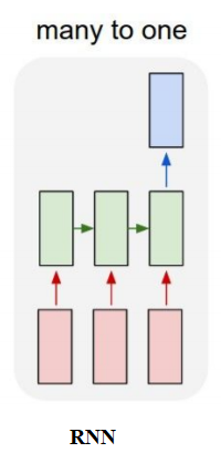
# [ 0, 0, 0, ..., 2, 316, 87]])Here we shall use a many-to-one RNN for sentiment analysis as shown below.
Build an LSTM model that takes a sentence as input and outputs the sentiment label.
model = Sequential()
model.add(Embedding(2000, 128,input_length = X.shape[1]))
model.add(SpatialDropout1D(0.3))
model.add(LSTM(128, dropout=0.2, recurrent_dropout=0.2))
model.add(Dense(2,activation='softmax'))
model.compile(loss = 'categorical_crossentropy', optimizer='adam',metrics = ['accuracy'])
print(model.summary())

_________________________________________________________________
Layer (type)                 Output Shape              Param #
=================================================================
embedding_10 (Embedding)     (None, 12, 128)           256000
_________________________________________________________________
spatial_dropout1d_10 (Spatia (None, 12, 128)           0
_________________________________________________________________
lstm_10 (LSTM)               (None, 128)               131584
_________________________________________________________________
dense_10 (Dense)             (None, 2)                 258
=================================================================
Total params: 387,842
Trainable params: 387,842
Non-trainable params: 0
_________________________________________________________________
None
Divide the dataset into train and validation (test) dataset and train the LSTM model on the dataset.
Y = pd.get_dummies(df['sentiment']).values
X_train, X_test, Y_train, Y_test, _, indices = train_test_split(X,Y, np.arange(len(X)), test_size = 0.33, random_state = 5)
model.fit(X_train, Y_train, epochs = 5, batch_size=32, verbose = 2)

#Epoch 1/5  - 3s - loss: 0.6748 - acc: 0.5522
#Epoch 2/5  - 1s - loss: 0.5358 - acc: 0.7925
#Epoch 3/5  - 1s - loss: 0.2368 - acc: 0.9418
#Epoch 4/5  - 1s - loss: 0.1011 - acc: 0.9761
#Epoch 5/5  - 1s - loss: 0.0578 - acc: 0.9836
Predict the sentiment labels of the (held out) test dataset.
result = model.predict(X[indices],batch_size=1,verbose = 2)
df1 = df.iloc[indices]
df1['neg_prob'] = result[:,0]
df1['pos_prob'] = result[:,1]
df1['pred'] = np.array(['negative', 'positive'])[np.argmax(result, axis=1)]
df1.head()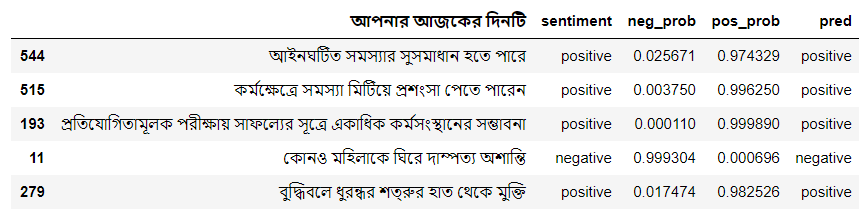
Finally, compute the accuracy of the model for the positive and negative ground-truth sentiment corresponding to daily astrological predictions.
df2 = df1[df1.sentiment == 'positive']
print('positive accuracy:' + str(np.mean(df2.sentiment == df2.pred)))
#positive accuracy:0.9177215189873418
df2 = df1[df1.sentiment == 'negative']
print('negative accuracy:' + str(np.mean(df2.sentiment == df2.pred)))
#negative accuracy:0.9352941176470588
Building a very simple Bangla Chatbot with RASA NLU
The following figure shows how to design a very simple Bangla chatbot to order food from restaurants using RASA NLU.
We need to design the intents, entities and slots to extract the entities properly and then design stories to define how the chatbot will respond to user inputs (core / dialog).
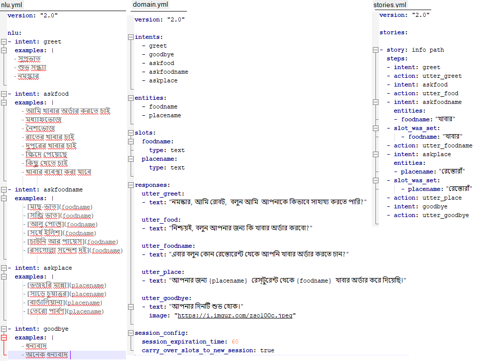
The following figure shows how the nlu, domain and stories files are written for the simple chatbot.
A sequence-to-sequence deep learning model is trained under the hood for intent classification. The next code block shows how the model can be trained.
import rasa
model_path = rasa.train('domain.yml', 'config.yml', ['data/'], 'models/')
The following gif demonstrates how the chatbot responds to user inputs.

References


Comments