

Graph Algorithms with Python
- Sandipan Dey

- Oct 10, 2020
- 13 min read
Updated: Oct 22, 2020
In this blog we shall discuss about a few popular graph algorithms and their python implementations. The problems discussed here appeared as programming assignments in the coursera course Algorithms on Graphs and on Rosalind. The problem statements are taken from the course itself. The basic building blocks of graph algorithms such as computing the number of connected components, checking whether there is a path between the given two vertices, checking whether there is a cycle, etc. are used practically in many applications working with graphs: for example, finding shortest paths on maps, analyzing social networks, analyzing biological data. For all the problems it can be assumed that the given input graph is simple, i.e., it does not contain self-loops (edges going from a vertex to itself) and parallel edges.
Checking if two vertices are Reachable
Given an undirected graph G=(V,E) and two distinct vertices 𝑢 and 𝑣, check if there is a path between 𝑢 and 𝑣. Steps
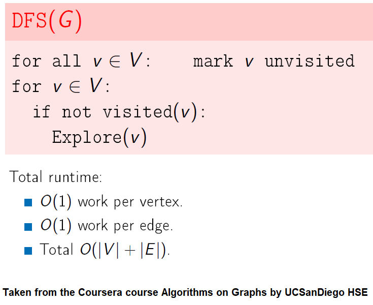
Starting from the node u, we can simply use breadth first search (bfs) or depth-first search (dfs) to explore the nodes reachable from u.
As soon as we find v we can return the nodes are reachable from one-another.
If v is not there in the nodes explored, we can conclude v is not reachable from u.
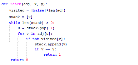
The following implementation (demonstrated using the following animations) uses iterative dfs (with stack) to check if two nodes (initially colored pink) are reachable.
We can optionally implement coloring of the nodes w.r.t. the following convention: initially the nodes are all white, when they are visited (pushed onto stack) they are marked as gray and finally when all the adjacent (children) nodes for a given node are visited, the node can be marked black.
We can store the parent of each node in an array and we can extract the path between two given nodes using the parent array, if they are reachable.
A very basic python implementation of the iterative dfs is shown below (here adj represents the adjacency list representation of the input graph):
The following animations demonstrate how the algorithm works, the stack is also shown at different points in time during the execution. Finally the path between the nodes are shown if they are reachable.
The same algorithm can be used for finding an Exit from a Maze (check whether there is a path from a given cell to a given exit).
Find Connected Components in an Undirected Graph
Given an undirected graph with 𝑛 vertices and 𝑚 edges, compute the number of connected components in it.
Steps
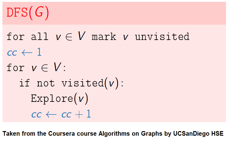
The following simple modification in dfs can be used to find the number of connected components in an undirected graph, as shown in the following figure.
From each node we need to find all the nodes yet to be explored.
We can find the nodes in a given component by finding all the nodes reachable from a given node.
The same iterative dfs implementation was used (demonstrated with the animations below).
The nodes in a component found were colored using the same color.
The same algorithm can be used to decide that there are no dead zones in a maze, that is, that at least one exit is reachable from each cell.
Find an Euler Tour / Circuit in a Directed Graph
Given A directed graph that contains an Eulerian tour, where the graph is given in the form of an adjacency list.
Steps
While solving the famous Königsberg Bridge Problem, Euler proved that an Euler circuit in an undirected graph exists iff all its nodes have even degree.
For an Euler tour to exist in an undirected graph, if there exists odd-degree nodes in the graph, there must be exactly 2 nodes with odd degrees - the tour will start from one such node and end in another node.
The tour must visit all the edges in the graph exactly once.
The degree test can be extended to directed graphs (with in-degrees and out-degrees) and can be used to determine the existence of Euler tour / circuit in a Digraph.
Flury's algorithm can be used to iteratively remove the edges (selecting the edges not burning the bridges in the graph as much as possible) from the graph and adding them to the tour.
DFS can be modified to obtain the Euler tour (circuit) in a DiGraph.
The following figure shows these couple of algorithms for finding the Euler tour / circuit in a graph if one exists (note in the figure path is meant to indicate tour). We shall use DFS to find Euler tour.

The following code snippets represent the functions used to find Euler tour in a graph. Here, variables n and m represent the number of vertices and edges of the input DiGraph, respectively, whereas adj represents the corresponding adjacency list.
Python Code
def count_in_out_degrees(adj):
   n = len(adj)
   in_deg, out_deg = [0]*n, [0]*n
   for u in range(n):
      for v in adj[u]:
         out_deg[u] += 1
         in_deg[v] += 1
   return in_deg, out_deg

def get_start_if_Euler_tour_present(in_deg, out_deg):
    start, end, tour = None, None, True
    for i in range(len(in_deg)):
       d = out_deg[i] - in_deg[i]
       if abs(d) > 1:
      	  tour = False
	  break
       elif d == 1:
          start = i
       elif d == -1:
	  end = i
     tour = (start != None and end != None) or \
	    (start == None and end == None)
     if tour and start == None: # a circuit
	start = 0
     return (tour, start)

def dfs(adj, v, out_deg, tour):
    while out_deg[v] > 0:
       out_deg[v] -= 1
	dfs(adj, adj[v][out_deg[v]], out_deg, tour)
    tour[:] = [v] + tour

def compute_Euler_tour(adj):
    n, m = len(adj), sum([len(adj[i]) for i in range(len(adj))])
    in_deg, out_deg = count_in_out_degrees(adj)
    tour_present, start = get_start_if_Euler_tour_present(in_deg,
                                                         out_deg)
    if not tour_present:
       return None
    tour = []
    dfs(adj, start, out_deg, tour)
    if len(tour) == m+1:
       return tour
    return None
The following animations show how the algorithm works.
Cycle Detection in a Directed Graph
Check whether a given directed graph with 𝑛 vertices and 𝑚 edges contains a cycle.
The following figure shows the classification of the edges encountered in DFS:
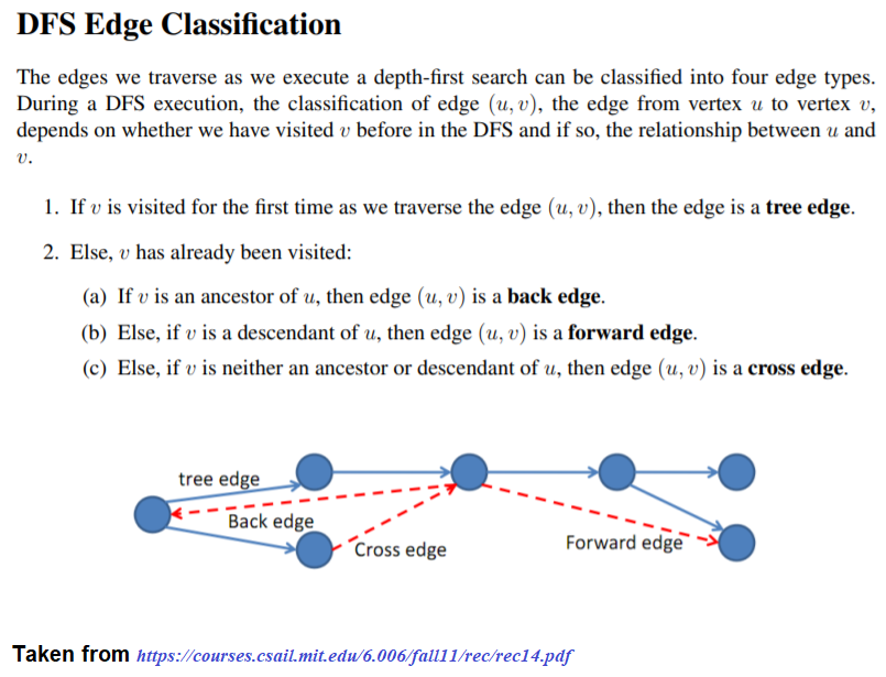
It can be shown that whether a Directed Graph is acyclic (DAG) or not (i.e. it contains a cycle), can be checked using the presence of a back-edge while DFS traversal.
Steps
Use the recursive DFS implementation (pseudo-code shown in the below figure)
Track if a node to be visited is already on the stack, if it's there, it forms a back edge.
Use parents array to obtain the directed cycle, if found.

The above algorithm can be used to check consistency in a curriculum (e.g., there is no cyclic dependency in the prerequisites for each course listed).
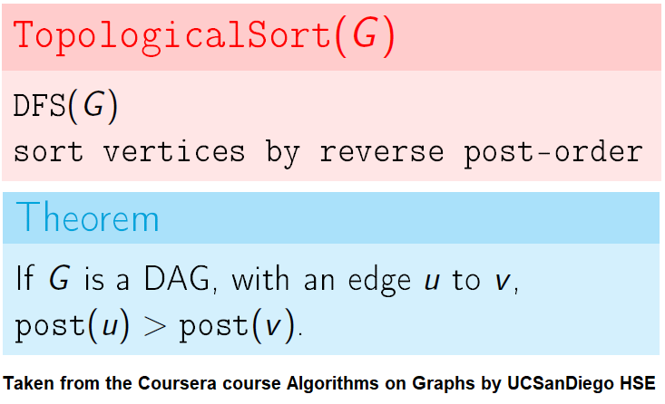
Topologically Order a Directed Graph
Compute a topological ordering of a given directed acyclic graph (DAG) with 𝑛 vertices and 𝑚 edges.
The intuitive idea can be to iteratively find a sink node v in the DiGraph G, put v at end of the desired order to be found and remove v from G, until G is empty. It can be done efficiently with DFS by keeping track of the time of pre and post visiting the nodes.
Steps
Use the recursive implementation of dfs.
When visiting a node with a recursive call, record the pre and post visit times, at the beginning and the end (once all the children of the given node already visited) of the recursive call, respectively.
Reorder the nodes by their post-visit times in descending order, as shown in the following figure.
The above algorithm can be used to determine the order of the courses in a curriculum, taking care of the pre-requisites dependencies.
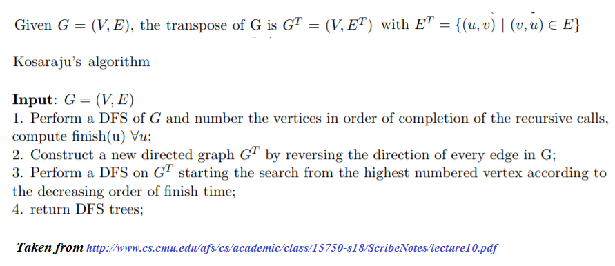
KosaRaju's Algorithm to find the Strongly Connected Components (SCC) in a Digraph
Compute the number of strongly connected components of a given directed graph with 𝑛 vertices and 𝑚 edges.
Note the following:
dfs can be used to find SCCs in a Digraph.
We need to make it sure that dfs traversal does not leave a such component with an outgoing edge.
The sink component is one that does not have an outgoing edge. We need to find a sink component first.
The vertex with the largest post-visit time is a source component for dfs.
The reverse (or transpose) graph of G has same SCC as the original graph.
Source components of the transpose of G are sink components of G.
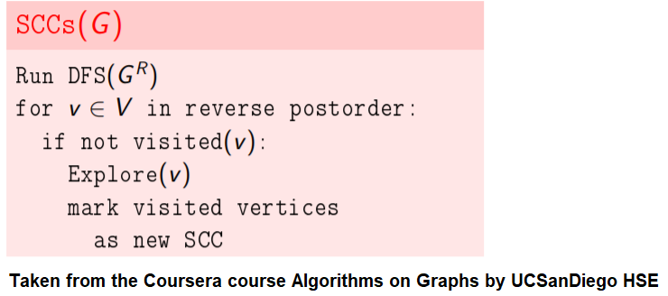
With all the above information, the following algorithm can be implemented to obtain the SCCs in a digraph G.
Alternatively, the algorithm can be represented as follows:
The following animations show how the algorithm works:

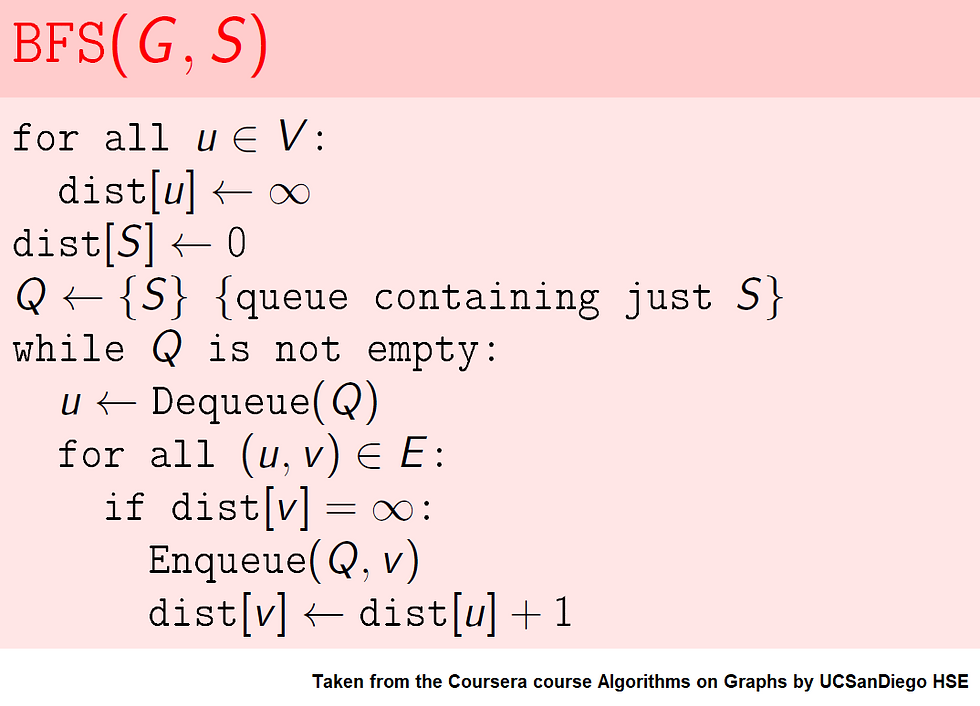
Shortest Path in an Undirected Graph with BFS
Given an undirected graph with 𝑛 vertices and 𝑚 edges and two vertices 𝑢 and 𝑣, compute the length of a shortest path between 𝑢 and 𝑣 (that is, the minimum number of edges in a path from 𝑢 to 𝑣).
The following figure shows the algorithm for bfs.
It uses a queue (FIFO) instead of a stack (LIFO) to store the nodes to be explored.
The traversal is also called level-order traversal, since the nodes reachable with smaller number of hops (shorter distances) from the source / start node are visited earlier than the higher-distance nodes.
The running time of bfs is again O(|E| + |V |).
The following animations demonstrate how the algorithm works.

Checking whether a Graph is Bipartite (2-Colorable)
Given an undirected graph with 𝑛 vertices and 𝑚 edges, check whether it is bipartite.
Steps
Note that a graph bipartite iff its vertices can be colored using 2 colors (so that no adjacent vertices have the same color).
Use bfs to traverse the graph from a starting node and color nodes in the alternate levels (measured by distances from source) with red (even level) and blue (odd level).
If at any point in time two adjacent vertices are found that are colored using the same color, then the graph is not 2-colorable (hence not bipartite).
If no such cases occur, then the graph is bipartite
For a graph with multiple components, use bfs on each of them.
Also, note that a graph is bipartite iff it contains an odd length cycle.
The following animations demonstrate how the algorithm works.
Notice that the last graph contained a length of cycle 4 (even length cycle) and it was bipartite graph. The graph prior to this one contained a triangle in it (cycle of odd length 3), it was not bipartite.
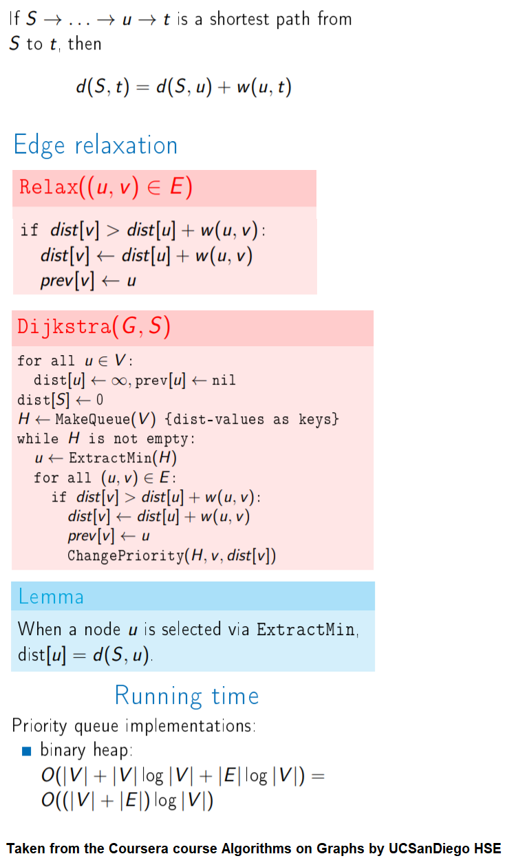
Shortest Path in an Weighted Graph with Dijkstra
Given an directed graph with positive edge weights and with 𝑛 vertices and 𝑚 edges as well as two
vertices 𝑢 and 𝑣, compute the weight of a shortest path between 𝑢 and 𝑣 (that is, the minimum total
weight of a path from 𝑢 to 𝑣).
Optimal substructure property : any subpath of an optimal path is also optimal.
Initially, we only know the distance to source node S and relax all the edges from S.
Maintain a set R of vertices for which dist is already set correctly (known region).
On each iteration take a vertex outside of R with the minimum dist-value, add it to R, and relax all its outgoing edges.
The next figure shows the pseudocode of the algorithm.
The following animations demonstrate how the algorithm works.
The algorithm works for the undirected graphs as well. The following animations show how the shortest path can be found on undirected graphs.
Detecting Negative Cycle in a Directed Graph with Bellman-Ford
Given an directed graph with possibly negative edge weights and with 𝑛 vertices and 𝑚 edges, check whether it contains a cycle of negative weight. Also given its vertex 𝑠, compute the length of shortest paths from 𝑠 to all other vertices of the graph.
Given an directed graph with possibly negative edge weights and with 𝑛 vertices and 𝑚 edges, check whether it contains a cycle of negative weight. Also, given a vertex 𝑠, compute the length of shortest paths from 𝑠 to all other vertices of the graph.
For a Digraph with n nodes (without a negative cycle), the shortest path length in between two nodes (e.g., the source node and any other node) can be at most n-1.
Relax edges while dist changes (at most n-1 times, most of the times the distances will stop changing much before that).
This algorithm works even for negative edge weights.
The following figure shows the pseudocode of the algorithm.

The above algorithm can also be used to detect a negative cycle in the input graph.
Run n = |V | iterations of Bellman–Ford algorithm (i.e., just run the edge-relaxation for once more, for the n-th time).
If there exists a vertex, the distance of which still decreases, it implies that there exist a negative-weight cycle in the graph and the vertex is reachable from that cycle.
Save node v relaxed on the last iteration v is reachable from a negative cycle
Start from x ← v, follow the link x ← prev[x] for |V | times — will be definitely on the cycle
Save y ← x and go x ← prev[x] until x = y again
The above algorithm can be used to detect infinite arbitrage, with the following steps:
Do |V | iterations of Bellman–Ford, save all nodes relaxed on V-th iteration-set A
Put all nodes from A in queue Q
Do breadth-first search with queue Q and find all nodes reachable from A
All those nodes and only those can have infinite arbitrage
The following animations demonstrate how the algorithm works.
The last animation shows how the shortest paths can be computed with the algorithm in the presence of negative edge weights.
Find Minimum Spanning Tree in a Graph with Prim's Greedy Algorithm
Given 𝑛 points on a plane, connect them with segments of minimum total length such that there is a path between any two points.
Steps
Let’s construct the following undirected graph G=(V, E): each node (in V) in the graph corresponds to a point in the plane and the weight of an edge (in E) in between any two nodes corresponds to the distance between the nodes.
The length of a segment with endpoints (𝑥1, 𝑦1) and (𝑥2, 𝑦2) is equal to the Euclidean distance √︀((𝑥1 − 𝑥2)² + (𝑦1 − 𝑦2)²).
Then the problem boils down to finding a Minimum Spanning Tree in the graph G.
The following figure defines the MST problem and two popular greedy algorithms Prim and Kruskal to solve the problem efficiently.
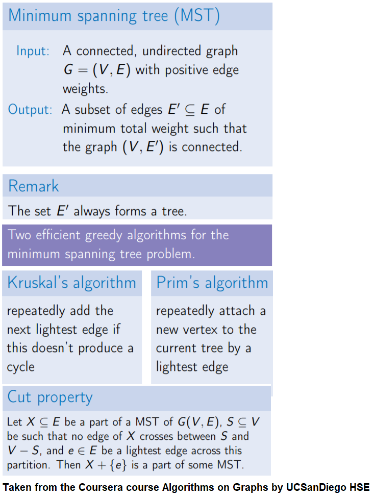
We shall use Prim’s algorithm to find the MST in the graph. Here are the algorithm steps:
It starts with an initial vertex and is grown to a spanning tree X.
X is always a subtree, grows by one edge at each iteration
Add a lightest edge between a vertex of the tree and a vertex not in the tree
Very similar to Dijkstra’s algorithm
The pseudocode is shown in the following figure.

The following animations demonstrate how the algorithm works for a few different set of input points in 2-D plane.
The following two animations show the algorithm steps on the input points and the corresponding graph formed, respectively.
The following animation shows how Prim’s algorithm outputs an MST for 36 input points in a 6x6 grid.
As expected, the cost of the MCST formed is 35 for the 36 points, since a spanning tree with n nodes has n-1 edges, each with unit length.
The above algorithm can be used to build roads between some pairs of the given cities such that there is a path between any two cities and the total length of the roads is minimized.
Finding Minimum Spanning Tree and Hierarchical Clustering with Kruskal
Given 𝑛 points on a plane and an integer 𝑘, compute the largest possible value of 𝑑 such that the
given points can be partitioned into 𝑘 non-empty subsets in such a way that the distance between any two points from different subsets is at least 𝑑.
Steps
We shall use Kruskal’s algorithm to solve the above problem. Each point can be thought of a node in the graph, as earlier, with the edge weights between the nodes being equal to the Euclidean distance between them.
Start with n components, each node representing one.
Run iterations of the Kruskal’s algorithm and merge the components till there are exactly k (< n) components left.
These k components will be the k desired clusters of the points and we can compute d to be the largest distance in between two points belonging to different clusters.
Here are the steps for the Kruskal’s algorithm to compute MST:
Start with each node in the graph as a single-node tree in a forest X.
Repeatedly add to X the next lightest edge e that doesn’t produce a cycle.
At any point of time, the set X is a forest (i.e., a collection of trees)
The next edge e connects two different trees — say, T1 and T2
The edge e is the lightest between T1 and V / T1, hence adding e is safe
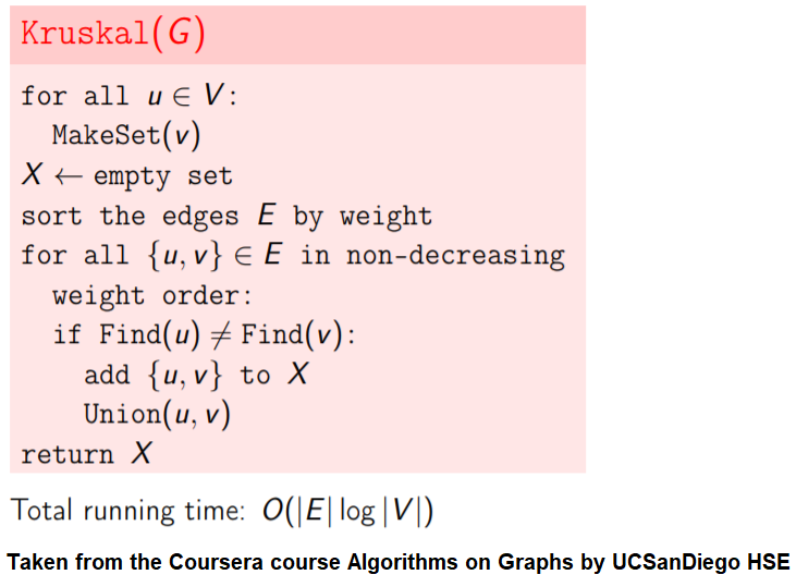
Use disjoint sets data structure for implementation
Initially, each vertex lies in a separate set
Each set is the set of vertices of a connected component
To check whether the current edge {u, v} produces a cycle, we check whether u and v belong to the same set (find).
Merge two sets using union operation.
The following figure shows a few algorithms to implement union-find abstractions for disjoint sets.

The following animations demonstrate how the algorithm works. Next couple of animations show how 8 points in a plane are (hierarchically) clustered using Kruskal’s algorithm and finally the MST is computed. The first animation shows how the points are clustered and the next one shows how Kruskal works on the corresponding graph created from the points.
The next animation again shows how a set of points in 2-D are clustered using Kruskal and MST is computed.
Clustering is a fundamental problem in data mining. The goal is to partition a given set of objects into subsets (or clusters) in such a way that any two objects from the same subset are close (or similar) to each other, while any two objects from different subsets are far apart.
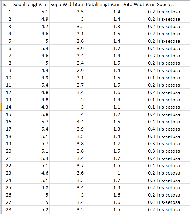
Now we shall use Kruskal’s algorithm to cluster a small real-world dataset named the Iris dataset (can be downloaded from the UCI Machine learning repository), often used as a test dataset in Machine learning.
Next 3 animations show how Kruskal can be used to cluster Iris dataset . The first few rows of the dataset are shown below:
Let’s use the first two features (SepalLength and SepalWidth), project the dataset in 2-D and use Kruskal to cluster the dataset, as shown in the following animation.
Now, let’s use the second and third feature variables (SepalWidth and PetalLength), project the dataset in 2-D and use Kruskal to cluster the dataset, as shown in the following animation.

Finally, let’s use the third and fourth feature variables (PetalLength and PetalWidth), project the dataset in 2-D and use Kruskal to cluster the dataset, as shown in the following animation.
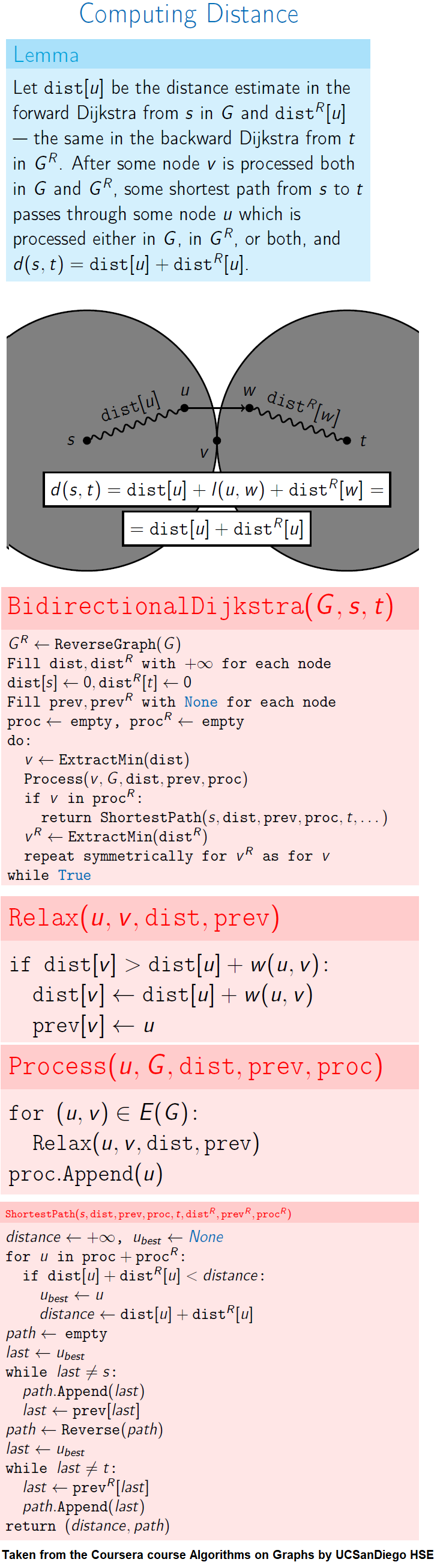
Friend Suggestion in Social Networks - Bidirectional Dijkstra
Compute the distance between several pairs of nodes in the network.
Steps
Build reverse graph GR
Start Dijkstra from s in G and from t in GR
Alternate between Dijkstra steps in G and in GR
Stop when some vertex v is processed both in G and in GR
Compute the shortest path between s and t
Meet-in-the-middle
More general idea, not just for graphs
Instead of searching for all possible objects, search for first halves and for second halves separately
Then find “compatible” halves
Typically roughly O(√N) instead of O(N)
Friends suggestions in social networks
Find the shortest path from Michael to Bob via friends connections
For the two “farthest” people, Dijkstra has to look through 2 billion people
If we only consider friends of friends of friends for both Michael and Bob, we will find a connection
Roughly 1M friends of friends of friends
1M + 1M = 2M people - 1000 times less
Dijkstra goes in circles
Bidirectional search idea can reduce the search space
Bidirectional Dijkstra can be 1000s times faster than Dijkstra for social networks
The following figure shows the algorithm
The following animation shows how the algorithm works:
Computing Distance Faster Using Coordinates with A* search
Compute the distance between several pairs of nodes in the network. The length l between any two nodes u an v is guaranteed to satisfy 𝑙 ≥ √︀((𝑥(𝑢) − 𝑥(𝑣))2 + (𝑦(𝑢) − 𝑦(𝑣))2).
Let's say we are submitting a query to find a shortest path between nodes (s,t) to a graph.
A potential function 𝜋(v) for a node v in a is an estimation of d(v, t) - how far is it from here to t?
If we have such estimation, we can often avoid going wrong direction directed search
Take some potential function 𝜋 and run Dijkstra algorithm with edge weights ℓ𝜋
For any edge (u, v), the new length ℓ𝜋(u, v) must be non-negative, such 𝜋 is called feasible
Typically 𝜋(v) is a lower bound on d(v, t)
A* is a directed search algorithm based on Dijkstra and potential functions
Run Dijkstra with the potential 𝜋 to find the shortest path - the resulting algorithm is A* search, described in the following figure
On a real map a path from v to t cannot be shorter than the straight line segment from v to t
For each v, compute 𝜋(v) = dE (v, t)
If 𝜋(v) gives lower bound on d(v, t)
Worst case: 𝜋(v) = 0 for all v the same as Dijkstra
Best case: 𝜋(v) = d(v, t) for all v then ℓ𝜋(u, v) = 0 iff (u, v) is on a shortest path to t, so search visits only the edges of shortest s − t paths
It can be shown that the tighter are the lower bounds the fewer vertices will be scanned

The following animations show how the A* search algorithm works on road networks (and the corresponding graph representations). Each node in the graph has the corresponding (distance, potential) pairs.
The following animations show how the shortest path is computed between two nodes for the USA road network for the San Francisco Bay area (the corresponding graph containing 321270 nodes and 800172 edges), using Dijkstra, bidirectional Dijkstra and A* algorithms respectively, the data can be downloaded from 9th DIMACS Implementation Challenge - Shortest Paths.


Comments