

Solving a few AI problems with Python
- Sandipan Dey

- Oct 10, 2020
- 47 min read
Updated: Oct 28, 2020
AI Problems on Search, Logic, Uncertainty, Optimization, Learning and Language
In this blog we shall discuss about a few problems in artificial intelligence and their python implementations. The problems discussed here appeared as programming assignments in the edX course CS50’s Introduction to Artificial Intelligence with Python (HarvardX:CS50 AI). The problem statements are taken from the course itself.
Degrees
Write a program that determines how many “degrees of separation” apart two actors are.
According to the Six Degrees of Kevin Bacon game, anyone in the Hollywood film industry can be connected to Kevin Bacon within six steps, where each step consists of finding a film that two actors both starred in.
In this problem, we’re interested in finding the shortest path between any two actors by choosing a sequence of movies that connects them. For example, the shortest path between Jennifer Lawrence and Tom Hanks is 2: Jennifer Lawrence is connected to Kevin Bacon by both starring in “X-Men: First Class,” and Kevin Bacon is connected to Tom Hanks by both starring in “Apollo 13.”
We can frame this as a search problem: our states are people. Our actions are movies, which take us from one actor to another (it’s true that a movie could take us to multiple different actors, but that’s okay for this problem).
Our initial state and goal state are defined by the two people we’re trying to connect. By using breadth-first search, we can find the shortest path from one actor to another.
The following figure shows how small samples from the dataset look like:
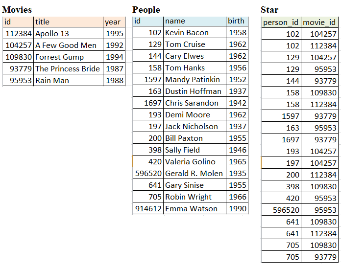
In the csv file for the people, each person has a unique id, corresponding with their id in IMDb’s database. They also have a name, and a birth year.
In the csv file for the movies, each movie also has a unique id, in addition to a title and the year in which the movie was released.
The csv file for the stars establishes a relationship between the people and the movies from the corresponding files. Each row is a pair of a person_id value and movie_id value.
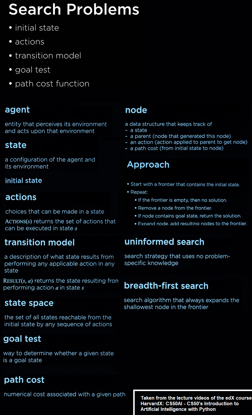
Given two actors nodes in the graph we need to find the distance (shortest path) between the nodes. We shall use BFS to find the distance or the degree of separation. The next figure shows the basic concepts required to define a search problem in AI.
The next python code snippet implements BFS and returns the path between two nodes source and target in the given input graph.
def shortest_path(source, target):
    """
    Returns the shortest list of (movie_id, person_id) pairs
    that connect the source to the target.
    If no possible path, returns None.
    """

    explored = set([])
    frontier = [source]
    parents = {}
    while len(frontier) > 0:
        person = frontier.pop(0)
        if person == target:
            break
        explored.add(person)
        for (m, p) in neighbors_for_person(person):
            if not p in frontier and not p in explored:
                frontier.append(p)
                parents[p] = (m, person)
    if not target in parents:
        return None
    path = []
    person = target
    while person != source:
        m, p = parents[person]
        path.append((m, person))
        person = p
    path = path[::-1]
    return path
The following animation shows how BFS finds the minimum degree(s) of separation (distance) between the query source and target actor nodes (green colored). The shortest path found between the actor nodes (formed of the edges corresponding to the movies a pair of actors acted together in) is colored in red.
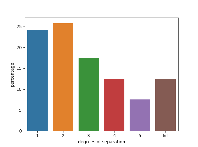
The following shows the distribution of the degrees of separation between the actors.
Tic-Tac-Toe
Using Minimax, implement an AI to play Tic-Tac-Toe optimally.
For this problem, the board is represented as a list of three lists (representing the three rows of the board), where each internal list contains three values that are either X, O, or EMPTY.
Implement a player function that should take a board state as input, and return which player’s turn it is (either X or O).
In the initial game state, X gets the first move. Subsequently, the player alternates with each additional move.
Any return value is acceptable if a terminal board is provided as input (i.e., the game is already over).
Implement an action function that should return a set of all of the possible actions that can be taken on a given board.
Each action should be represented as a tuple (i, j) where i corresponds to the row of the move (0, 1, or 2) and j corresponds to which cell in the row corresponds to the move (also 0, 1, or 2).
Possible moves are any cells on the board that do not already have an X or an O in them.
Any return value is acceptable if a terminal board is provided as input.
Implement a result function that takes a board and an action as input, and should return a new board state, without modifying the original board.
If action is not a valid action for the board, your program should raise an exception.
The returned board state should be the board that would result from taking the original input board, and letting the player whose turn it is make their move at the cell indicated by the input action.
Importantly, the original board should be left unmodified: since Minimax will ultimately require considering many different board states during its computation. This means that simply updating a cell in board itself is not a correct implementation of the result function. You’ll likely want to make a deep copy of the board first before making any changes.
Implement a winner function that should accept a board as input, and return the winner of the board if there is one.
If the X player has won the game, your function should return X. If the O player has won the game, your function should return O.
One can win the game with three of their moves in a row horizontally, vertically, or diagonally.
You may assume that there will be at most one winner (that is, no board will ever have both players with three-in-a-row, since that would be an invalid board state).
If there is no winner of the game (either because the game is in progress, or because it ended in a tie), the function should return None.
Implement a terminal function that should accept a board as input, and return a boolean value indicating whether the game is over.
If the game is over, either because someone has won the game or because all cells have been filled without anyone winning, the function should return True.
Otherwise, the function should return False if the game is still in progress.
Implement an utility function that should accept a terminal board as input and output the utility of the board.
If X has won the game, the utility is 1. If O has won the game, the utility is -1. If the game has ended in a tie, the utility is 0.
You may assume utility will only be called on a board if terminal(board) is True.
Implement a minimax function that should take a board as input, and return the optimal move for the player to move on that board.
The move returned should be the optimal action (i, j) that is one of the allowable actions on the board. If multiple moves are equally optimal, any of those moves is acceptable.
If the board is a terminal board, the minimax function should return None.
For all functions that accept a board as input, you may assume that it is a valid board (namely, that it is a list that contains three rows, each with three values of either X, O, or EMPTY).
Since Tic-Tac-Toe is a tie given optimal play by both sides, you should never be able to beat the AI (though if you don’t play optimally as well, it may beat you!)
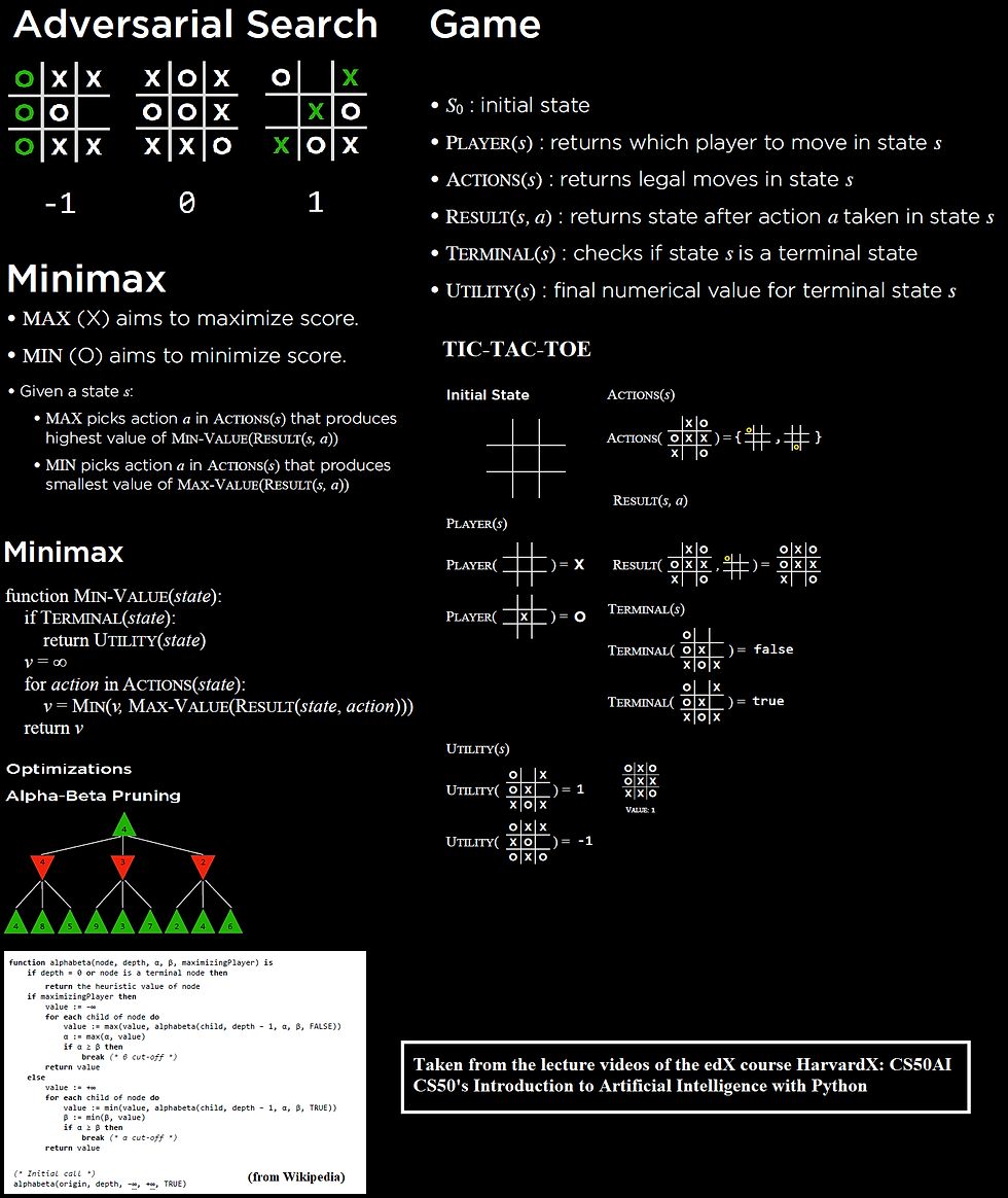
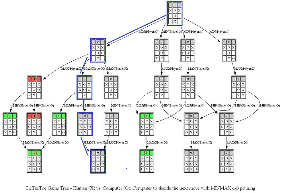
The following figure demonstrates the basic concepts of adversarial search and Game and defines the different functions for tic-tac-toe.
Here we shall use Minimax with alpha-beta pruning to speedup the game when it is computer’s turn.
The following python code fragment shows how to implement the minimax algorithm with alpha-beta pruning:
def max_value_alpha_beta(board, alpha, beta):
if terminal(board):
return utility(board), None
v, a = -np.inf, None
for action in actions(board):
m, _ = min_value_alpha_beta(result(board, action),
alpha, beta)
if m > v:
v, a = m, action
alpha = max(alpha, v)
if alpha >= beta:
break
return (v, a)
def min_value_alpha_beta(board, alpha, beta):
if terminal(board):
return utility(board), None
v, a = np.inf, None
for action in actions(board):
m, _ = max_value_alpha_beta(result(board, action),
alpha, beta)
if m < v:
v, a = m, action
beta = min(beta, v)
if alpha >= beta:
break
return (v, a)
def minimax(board):
"""
Returns the optimal action for the current player on the board.
"""
if terminal(board):
return None
cur_player = player(board)
if cur_player == X:
_, a = max_value_alpha_beta(board, -np.inf, np.inf)
elif cur_player == O:
_, a = min_value_alpha_beta(board, -np.inf, np.inf)
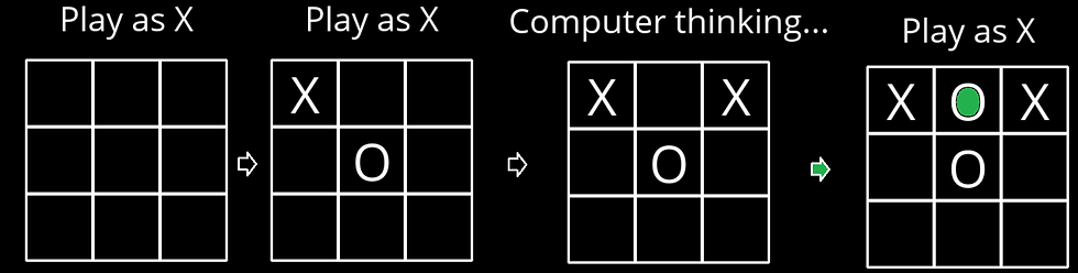
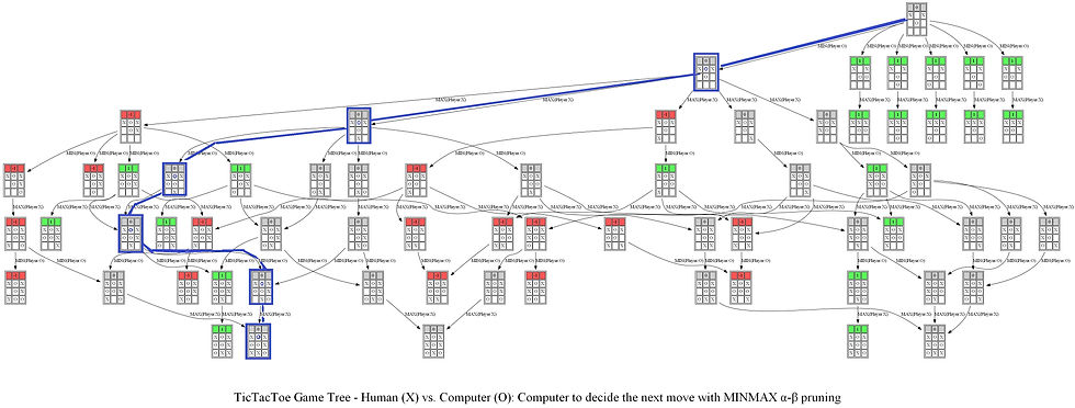
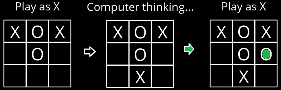
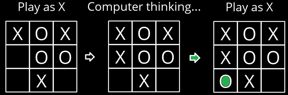
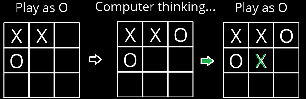
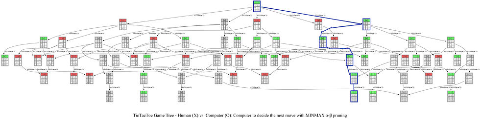
return aThe following sequence of actions by the human player (plays as X, the Max player) and the computer (plays as O, the Min player) shows what the computer thinks to come up with optimal position of O and the game tree it produces using Minimax with alpha-beta pruning algorithm shown in the above figure.
The following animations show how the game tree is created when the computer thinks for the above turn. The row above the game board denotes the value of the utility function and it’s color-coded: when the value of the corresponding state is +1 (in favor of the Max player) it’s colored as green, when the value is -1 (in favor of the Min player) it’s colored as red, otherwise it’s colored gray if the value is 0.
Notice the game tree is full-grown to the terminal leaves. The following figure shows a path (colored in blue) in the game tree that leads to a decision taken by the computer to choose the position of O.
Now let’s consider the next sequence of actions by the human player and the computer. As can be seen, the computer again finds the optimal position.
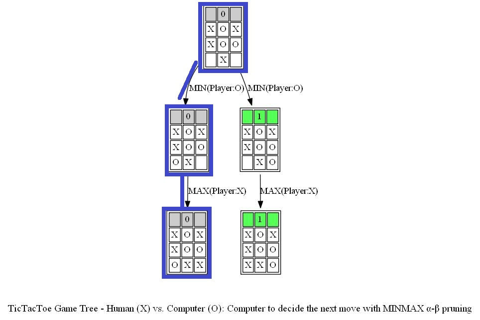
The following animation shows how the game tree is created when the computer thinks for the above turn.
The following figure shows a path (colored in blue) in the game tree that leads to a decision taken by the computer to choose the position of O (note that the optimal path corresponds to a tie in a terminal node).
Finally, let’s consider the next sequence of actions by the human player and the computer. As can be seen, the computer again finds the optimal position.
The following animations show how the game tree is created when the computer thinks for the above turn.
The next figure shows the path (colored in blue) in the game tree that leads to a decision taken by the computer to choose the position of O (note that the optimal path corresponds to a tie in a terminal node).
Now let’s consider another example game. The following sequence of actions by the computer player (AI agent now plays as X, the Max player) and the human player (plays as O, the Min player) shows what the computer thinks to come up with optimal position of O and the game tree it produces using Minimax with alpha-beta pruning algorithm.
The following animations show how the game tree is created when the computer thinks for the above turn.

The next figure shows the path (colored in blue) in the game tree that leads to a decision taken by the computer to choose the next position of X (note that the optimal path corresponds to a win in a terminal node).
Note from the above tree that no matter what action the human player chooses next, AI agent (the computer) can always win the game. An example final outcome of the game be seen from the next game tree.

Knights
Write a program to solve logic puzzles.
In 1978, logician Raymond Smullyan published “What is the name of this book?”, a book of logical puzzles. Among the puzzles in the book were a class of puzzles that Smullyan called “Knights and Knaves” puzzles.
In a Knights and Knaves puzzle, the following information is given: Each character is either a knight or a knave.
A knight will always tell the truth: if knight states a sentence, then that sentence is true.
Conversely, a knave will always lie: if a knave states a sentence, then that sentence is false.
The objective of the puzzle is, given a set of sentences spoken by each of the characters, determine, for each character, whether that character is a knight or a knave.
The task in this problem is to determine how to represent these puzzles using propositional logic, such that an AI running a model-checking algorithm could solve these puzzles.
Puzzles
Contains a single character: A. - A says “I am both a knight and a knave.”
Has two characters: A and B. - A says “We are both knaves.” - B says nothing.
Has two characters: A and B. - A says “We are the same kind.” - B says “We are of different kinds.”
Has three characters: A, B, and C. - A says either “I am a knight.” or “I am a knave.”, but you don’t know which. - B says “A said ‘I am a knave.’” - B then says “C is a knave.” - C says “A is a knight.”
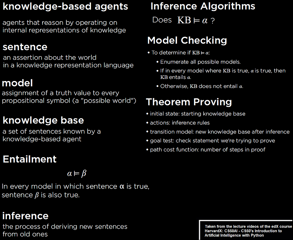
In this problem, we shall use model checking to find the solutions to the above puzzles. The following figure shows the theory that are relevant.
The following python code snippet shows the base class corresponding to a propositional logic sentence (taken from the code provided for the assignment).
import itertoolsclass Sentence():    def evaluate(self, model):
        """Evaluates the logical sentence."""
        raise Exception("nothing to evaluate")    def formula(self):
        """Returns string formula representing logical sentence."""
        return ""    def symbols(self):
        """Returns a set of all symbols in the logical sentence."""
        return set()    @classmethod
    def validate(cls, sentence):
        if not isinstance(sentence, Sentence):
            raise TypeError("must be a logical sentence")
Now, a propositional symbol and an operator (unary / binary) can inherit this class and implement the methods specific to the symbol as shown for the boolean operator AND (the code taken from the resources provided for the assignment).
class And(Sentence):
    def __init__(self, *conjuncts):
        for conjunct in conjuncts:
            Sentence.validate(conjunct)
        self.conjuncts = list(conjuncts)

    def __eq__(self, other):
        return isinstance(other, And) and \
               self.conjuncts == other.conjuncts

    def __hash__(self):
        return hash(
            ("and", tuple(hash(conjunct) for conjunct in
                         self.conjuncts))
        )

    def __repr__(self):
        conjunctions = ", ".join(
            [str(conjunct) for conjunct in self.conjuncts]
        )
        return f"And({conjunctions})"

    def add(self, conjunct):
        Sentence.validate(conjunct)
        self.conjuncts.append(conjunct)

    def evaluate(self, model):
        return all(conjunct.evaluate(model) for conjunct in
                   self.conjuncts)    def formula(self):
        if len(self.conjuncts) == 1:
            return self.conjuncts[0].formula()
        return " ∧ ".join([Sentence.parenthesize(conjunct.formula())
                           for conjunct in self.conjuncts])

    def symbols(self):
        return set.union(*[conjunct.symbols() \
               for conjunct in self.conjuncts])
Finally, we need to represent the KB for every puzzle, as the one shown in the code below:
AKnight = Symbol("A is a Knight")
AKnave = Symbol("A is a Knave")BKnight = Symbol("B is a Knight")
BKnave = Symbol("B is a Knave")CKnight = Symbol("C is a Knight")
CKnave = Symbol("C is a Knave")# Puzzle 1
# A says "I am both a knight and a knave."
knowledge0 = And(
    # TODO
    Or(And(AKnight, Not(AKnave)), And(Not(AKnight), AKnave)),
    Implication(AKnight, And(AKnight, AKnave)),
    Implication(AKnave, Not(And(AKnight, AKnave)))
)
The following section demonstrates the outputs obtained with model checking implemented using the above code (by iteratively assigning all possible models / truth values and checking if the KB corresponding to a puzzle evaluates to true for a model, and then outputting all the models for which the KB evaluates to true). To start solving a puzzle we must define the KB for the puzzle as shown above.
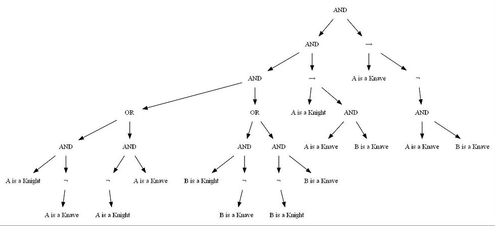
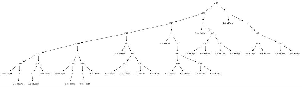
The following figure shows the KB (presented in terms of a propositional logic sentence and) shown as an expression tree for the Puzzle 1.

The following animation shows how model-checking solves Puzzle 1 (the solution is marked in green).
The following figure shows the KB in terms of an expression tree for the Puzzle 2
The following animation shows how model-checking solves Puzzle 2 (the solution is marked in green).
The following figure shows the KB in terms of an expression tree for the Puzzle 3
The following animation shows how model-checking solves Puzzle 3 (the solution is marked in green).

The following figure shows the KB in terms of an expression tree for the Puzzle 4
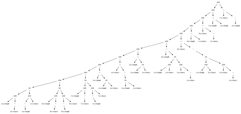
The following animation shows how model-checking solves Puzzle 4 (the solution is marked in green).
Minesweeper
Write an AI agent to play Minesweeper.
Minesweeper is a puzzle game that consists of a grid of cells, where some of the cells contain hidden “mines.”
Clicking on a cell that contains a mine detonates the mine, and causes the user to lose the game.
Clicking on a “safe” cell (i.e., a cell that does not contain a mine) reveals a number that indicates how many neighboring cells — where a neighbor is a cell that is one square to the left, right, up, down, or diagonal from the given cell — contain a mine.
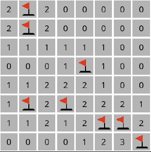
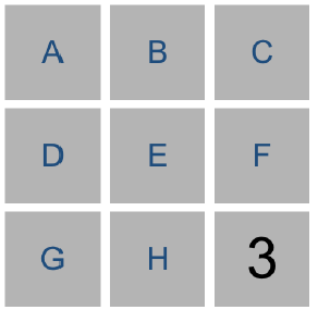
The following figure shows an example Minesweeper game. In this 3 X 3 Minesweeper game, for example, the three 1 values indicate that each of those cells has one neighboring cell that is a mine. The four 0 values indicate that each of those cells has no neighboring mine.
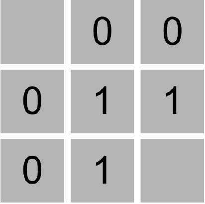
Given this information, a logical player could conclude that there must be a mine in the lower-right cell and that there is no mine in the upper-left cell, for only in that case would the numerical labels on each of the other cells be accurate.
The goal of the game is to flag (i.e., identify) each of the mines.
In many implementations of the game, the player can flag a mine by right-clicking on a cell (or two-finger clicking, depending on the computer).
Propositional Logic
Your goal in this project will be to build an AI that can play Minesweeper. Recall that knowledge-based agents make decisions by considering their knowledge base, and making inferences based on that knowledge.
One way we could represent an AI’s knowledge about a Minesweeper game is by making each cell a propositional variable that is true if the cell contains a mine, and false otherwise.
What information does the AI agent have access to? Well, the AI would know every time a safe cell is clicked on and would get to see the number for that cell.
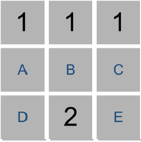
Consider the following Minesweeper board, where the middle cell has been revealed, and the other cells have been labeled with an identifying letter for the sake of discussion.
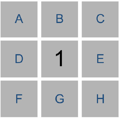
What information do we have now? It appears we now know that one of the eight neighboring cells is a mine. Therefore, we could write a logical expression like the following one to indicate that one of the neighboring cells is a mine: Or(A, B, C, D, E, F, G, H)
But we actually know more than what this expression says. The above logical sentence expresses the idea that at least one of those eight variables is true. But we can make a stronger statement than that: we know that exactly one of the eight variables is true. This gives us a propositional logic sentence like the below.
Or(
And(A, Not(B), Not(C), Not(D), Not(E), Not(F), Not(G), Not(H)),
And(Not(A), B, Not(C), Not(D), Not(E), Not(F), Not(G), Not(H)),
And(Not(A), Not(B), C, Not(D), Not(E), Not(F), Not(G), Not(H)),
And(Not(A), Not(B), Not(C), D, Not(E), Not(F), Not(G), Not(H)),
And(Not(A), Not(B), Not(C), Not(D), E, Not(F), Not(G), Not(H)),
And(Not(A), Not(B), Not(C), Not(D), Not(E), F, Not(G), Not(H)),
And(Not(A), Not(B), Not(C), Not(D), Not(E), Not(F), G, Not(H)),
And(Not(A), Not(B), Not(C), Not(D), Not(E), Not(F), Not(G), H)
)
That’s quite a complicated expression! And that’s just to express what it means for a cell to have a 1 in it. If a cell has a 2 or 3 or some other value, the expression could be even longer.
Trying to perform model checking on this type of problem, too, would quickly become intractable: on an 8 X 8 grid, the size Microsoft uses for its Beginner level, we’d have 64 variables, and therefore 2⁶⁴ possible models to check — far too many for a computer to compute in any reasonable amount of time. We need a better representation of knowledge for this problem.
Knowledge Representation
Instead, we’ll represent each sentence of our AI’s knowledge like the below. {A, B, C, D, E, F, G, H} = 1
Every logical sentence in this representation has two parts: a set of cells on the board that are involved in the sentence, and a number count , representing the count of how many of those cells are mines. The above logical sentence says that out of cells A, B, C, D, E, F, G, and H, exactly 1 of them is a mine.
Why is this a useful representation? In part, it lends itself well to certain types of inference. Consider the game below:
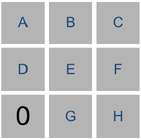
Using the knowledge from the lower-left number, we could construct the sentence {D, E, G} = 0 to mean that out of cells D, E, and G, exactly 0 of them are mines.
Intuitively, we can infer from that sentence that all of the cells must be safe. By extension, any time we have a sentence whose count is 0 , we know that all of that sentence’s cells must be safe.
Similarly, consider the game below.
Our AI agent would construct the sentence {E, F, H} = 3 . Intuitively, we can infer that all of E, F, and H are mines.
More generally, any time the number of cells is equal to the count , we know that all of that sentence’s cells must be mines.
In general, we’ll only want our sentences to be about cells that are not yet known to be either safe or mines. This means that, once we know whether a cell is a mine or not, we can update our sentences to simplify them and potentially draw new conclusions.
For example, if our AI agent knew the sentence {A, B, C} = 2 , we don’t yet have enough information to conclude anything. But if we were told that C were safe, we could remove C from the sentence altogether, leaving us with the sentence {A, B} = 2 (which, incidentally, does let us draw some new conclusions.)
Likewise, if our AI agent knew the sentence {A, B, C} = 2 , and we were told that C is a mine, we could remove C from the sentence and decrease the value of count (since C was a mine that contributed to that count), giving us the sentence {A, B} = 1 . This is logical: if two out of A, B, and C are mines, and we know that C is a mine, then it must be the case that out of A and B, exactly one of them is a mine.
If we’re being even more clever, there’s one final type of inference we can do
Consider just the two sentences our AI agent would know based on the top middle cell and the bottom middle cell. From the top middle cell, we have {A, B, C} = 1 . From the bottom middle cell, we have {A, B, C, D, E} = 2 . Logically, we could then infer a new piece of knowledge, that {D, E} = 1 . After all, if two of A, B, C, D, and E are mines, and only one of A, B, and C are mines, then it stands to reason that exactly one of D and E must be the other mine.
More generally, any time we have two sentences set1 = count1 and set2 = count2 where set1 is a subset of set2 , then we can construct the new sentence set2 — set1 = count2 — count1 . Consider the example above to ensure you understand why that’s true.
So using this method of representing knowledge, we can write an AI agent that can gather knowledge about the Minesweeper board, and hopefully select cells it knows to be safe!
The following figure shows examples of inference rules and resolution by inference relevant for this problem:

A few implementation tips
Represent a logical sentence by a python class Sentence again.
Each sentence has a set of cells within it and a count of how many of those cells are mines.
Let the class also contain functions known_mines and known_safes for determining if any of the cells in the sentence are known to be mines or known to be safe.
It should also have member functions mark_mine() and mark_safe() to update a sentence in response to new information about a cell.
Each cell is a pair (i, j) where i is the row number (ranging from 0 to height — 1 ) and j is the column number (ranging from 0 to width — 1 ).
Implement a known_mines() method that should return a set of all of the cells in self.cells that are known to be mines.
Implement a known_safes() method that should return a set of all the cells in self.cells that are known to be safe.
Implement a mark_mine() method that should first check if cell is one of the cells included in the sentence. If cell is in the sentence, the function should update the sentence so that cell is no longer in the sentence, but still represents a logically correct sentence given that cell is known to be a mine.
Likewise mark_safe() method should first check if cell is one of the cells included in the sentence. If yes, then it should update the sentence so that cell is no longer in the sentence, but still represents a logically correct sentence given that cell is known to be safe.
Implement a method add_knowledge() that should accept a cell and
The function should mark the cell as one of the moves made in the game.
The function should mark the cell as a safe cell, updating any sentences that contain the cell as well.
The function should add a new sentence to the AI’s knowledge base, based on the value of cell and count , to indicate that count of the cell ’s neighbors are mines. Be sure to only include cells whose state is still undetermined in the sentence.
If, based on any of the sentences in self.knowledge , new cells can be marked as safe or as mines, then the function should do so.
If, based on any of the sentences in self.knowledge , new sentences can be inferred , then those sentences should be added to the knowledge base as well.
Implement a method make_safe_move() that should return a move (i, j) that is known to be safe.
The move returned must be known to be safe, and not a move already made.
If no safe move can be guaranteed, the function should return None .
Implement a method make_random_move() that should return a random move (i, j) .
This function will be called if a safe move is not possible: if the AI agent doesn’t know where to move, it will choose to move randomly instead.
The move must not be a move that has already been made.
he move must not be a move that is known to be a mine.
If no such moves are possible, the function should return None .
The following python code snippet shows implementation of few of the above functions:
class MinesweeperAI():
    """
    Minesweeper game player
    """    def mark_mine(self, cell):
        """
        Marks a cell as a mine, and updates all knowledge
        to mark that cell as a mine as well.
        """
        self.mines.add(cell)
        for sentence in self.knowledge:
            sentence.mark_mine(cell)    # ensure that no duplicate
                                        # sentences are added
    def knowledge_contains(self, sentence):
        for s in self.knowledge:
            if s == sentence:
               return True
        return False    def add_knowledge(self, cell, count):
        """
        Called when the Minesweeper board tells us, for a given
        safe cell, how many neighboring cells have mines in them.
        This function should:
            1) mark the cell as a move that has been made
            2) mark the cell as safe
            3) add a new sentence to the AI's knowledge base
               based on the value of `cell` and `count`
            4) mark any additional cells as safe or as mines
               if it can be concluded based on the AI's KB
            5) add any new sentences to the AI's knowledge base
               if they can be inferred from existing knowledge
        """
        # mark the cell as a move that has been made
        self.moves_made.add(cell)
        # mark the cell as safe
        self.mark_safe(cell)
        # add a new sentence to the AI's knowledge base,
        # based on the value of `cell` and `count
        i, j = cell
        cells = []
        for row in range(max(i-1,0), min(i+2,self.height)):
            for col in range(max(j-1,0), min(j+2,self.width)):
                # if some mines in the neighbors are already known,
                # make sure to decrement the count
                if (row, col) in self.mines:
                   count -= 1
                if (not (row, col) in self.safes) and \
                   (not (row, col) in self.mines):
                   cells.append((row, col))
        sentence = Sentence(cells, count)
        # add few more inference rules here

    def make_safe_move(self):
        """
        Returns a safe cell to choose on the Minesweeper board.
        The move must be known to be safe, and not already a move
        that has been made.
        This function may use the knowledge in self.mines,
        self.safes and self.moves_made, but should not modify any of
        those values.
        """
        safe_moves = self.safes - self.moves_made
        if len(safe_moves) > 0:
           return safe_moves.pop()
        else:
           return None
The following animations show how the Minesweeper AI agent updates safe / mine cells and updates its knowledge-base, for a few example games (the light green and red cells represent known safe and mine cells, respectively, in the 2nd subplot):
PageRank
Write an AI agent to rank web pages by importance.
When search engines like Google display search results, they do so by placing more “important” and higher-quality pages higher in the search results than less important pages. But how does the search engine know which pages are more important than other pages?
One heuristic might be that an “important” page is one that many other pages link to, since it’s reasonable to imagine that more sites will link to a higher-quality webpage than a lower-quality webpage.
We could therefore imagine a system where each page is given a rank according to the number of incoming links it has from other pages, and higher ranks would signal higher importance.
But this definition isn’t perfect: if someone wants to make their page seem more important, then under this system, they could simply create many other pages that link to their desired page to articially inate its rank.
For that reason, the PageRank algorithm was created by Google’s co-founders (including Larry Page, for whom the algorithm was named).
In PageRank’s algorithm, a website is more important if it is linked to by other important websites, and links from less important websites have their links weighted less.
This definition seems a bit circular, but it turns out that there are multiple strategies for calculating these rankings.
Random Surfer Model
One way to think about PageRank is with the random surfer model, which considers the behavior of a hypothetical surfer on the internet who clicks on links at random.
The random surfer model imagines a surfer who starts with a web page at random, and then randomly chooses links to follow.
A page’s PageRank, then, can be described as the probability that a random surfer is on that page at any given time. After all, if there are more links to a particular page, then it’s more likely that a random surfer will end up on that page.
Moreover, a link from a more important site is more likely to be clicked on than a link from a less important site that fewer pages link to, so this model handles weighting links by their importance as well.
One way to interpret this model is as a Markov Chain, where each page represents a state, and each page has a transition model that chooses among its links at random. At each time step, the state switches to one of the pages linked to by the current state.
By sampling states randomly from the Markov Chain, we can get an estimate for each page’s PageRank. We can start by choosing a page at random, then keep following links at random, keeping track of how many times we’ve visited each page.
After we’ve gathered all of our samples (based on a number we choose in advance), the proportion of the time we were on each page might be an estimate for that page’s rank.
To ensure we can always get to somewhere else in the corpus of web pages, we’ll introduce to our model a damping factor d .
With probability d (where d is usually set around 0.85 ), the random surfer will choose from one of the links on the current page at random. But otherwise (with probability 1 — d ), the random surfer chooses one out of all of the pages in the corpus at random (including the one they are currently on).
Our random surfer now starts by choosing a page at random, and then, for each additional sample we’d like to generate, chooses a link from the current page at random with probability d , and chooses any page at random with probability 1 — d .
If we keep track of how many times each page has shown up as a sample, we can treat the proportion of states that were on a given page as its PageRank.
Iterative Algorithm
We can also define a page’s PageRank using a recursive mathematical expression. Let PR(p) be the PageRank of a given page p : the probability that a random surfer ends up on that page.
How do we define PR(p)? Well, we know there are two ways that a random surfer could end up on the page: 1. With probability 1 — d , the surfer chose a page at random and ended up on page p . 2. With probability d , the surfer followed a link from a page i to page p .
The first condition is fairly straightforward to express mathematically: it’s 1 — d divided by N , where N is the total number of pages across the entire corpus. This is because the 1 — d probability of choosing a page at random is split evenly among all N possible pages.
For the second condition, we need to consider each possible page i that links to page p . For each of those incoming pages, let NumLinks(i) be the number of links on page i .
Each page i that links to p has its own PageRank, PR(i) , representing the probability that we are on page i at any given time.
And since from page i we travel to any of that page’s links with equal probability, we divide PR(i) by the number of links NumLinks(i) to get the probability that we were on page i and chose the link to page p.
This gives us the following definition for the PageRank for a page p .
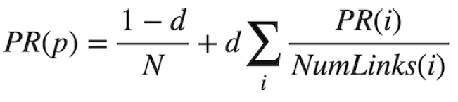
In this formula, d is the damping factor, N is the total number of pages in the corpus, i ranges over all pages that link to page p , and NumLinks(i) is the number of links present on page i .
How would we go about calculating PageRank values for each page, then? We can do so via iteration: start by assuming the PageRank of every page is 1 / N (i.e., equally likely to be on any page).
Then, use the above formula to calculate new PageRank values for each page, based on the previous PageRank values.
If we keep repeating this process, calculating a new set of PageRank values for each page based on the previous set of PageRank values, eventually the PageRank values will converge (i.e., not change by more than a small threshold with each iteration).
Now, let’s implement both such approaches for calculating PageRank — calculating both by sampling pages from a Markov Chain random surfer and by iteratively applying the PageRank formula.
The following python code snippet represents the implementation of PageRank computation with Monte-Carlo sampling.
def sample_pagerank(corpus, damping_factor, n):
    """
    Return PageRank values for each page by sampling `n` pages
    according to transition model, starting with a page at random.
    Return a dictionary where keys are page names, and values are
    their estimated PageRank value (a value between 0 and 1). All
    PageRank values should sum to 1.
    """
    pages = [page for page in corpus]
    pageranks = {page:0 for page in pages}
    page = random.choice(pages)
    pageranks[page] = 1
    for i in range(n):
        probs = transition_model(corpus, page, damping_factor)
        probs = probs.values() #[probs[p] for p in pages]
        page = random.choices(pages, weights=probs, k=1)[0]
        pageranks[page] += 1
    return {page:pageranks[page]/n for page in pageranks}
The following animation shows how PageRank changes with sampling-based implementation.
Again, the following python code snippet represents the iterative PageRank implementation.
def iterate_pagerank(corpus, damping_factor):
    """
    Return PageRank values for each page by iteratively updating
    PageRank values until convergence.    Return a dictionary where
    keys are page names, and values are their estimated PageRank value
    (a value between 0 and 1). All PageRank values should sum to 1.
    """
    incoming = {p:set() for p in corpus}
    for p in corpus:
        for q in corpus[p]:
           incoming[q].add(p)
    pages = [page for page in corpus]
    n = len(pages)
    pageranks = {page:1/n for page in pages}
    diff = float('inf')
    while diff > 0.001:
        diff = 0
        for page in pages:
            p = (1-damping_factor)/n
            for q in incoming[page]:
               p += damping_factor * \
                (sum([pageranks[q]/len(corpus[q])]) \
                if len(corpus[q]) > 0 else 1/n)
            diff = max(diff, abs(pageranks[page]-p))
            pageranks[page] = p
    return {p:pageranks[p]/sum(pageranks.values())
            for p in pageranks}
The following animation shows how the iterative PageRank formula is computed for a sample very small web graph:

Heredity
Write an AI agent to assess the likelihood that a person will have a particular genetic trait.
Mutated versions of the GJB2 gene are one of the leading causes of hearing impairment in newborns.
Each person carries two versions of the gene, so each person has the potential to possess either 0, 1, or 2 copies of the hearing impairment version GJB2.
Unless a person undergoes genetic testing, though, it’s not so easy to know how many copies of mutated GJB2 a person has.
This is some “hidden state”: information that has an effect that we can observe (hearing impairment), but that we don’t necessarily directly know.
After all, some people might have 1 or 2 copies of mutated GJB2 but not exhibit hearing impairment, while others might have no copies of mutated GJB2 yet still exhibit hearing impairment.
Every child inherits one copy of the GJB2 gene from each of their parents. If a parent has two copies of the mutated gene, then they will pass the mutated gene on to the child; if a parent has no copies of the mutated gene, then they will not pass the mutated gene on to the child; and if a parent has one copy of the mutated gene, then the gene is passed on to the child with probability 0.5.
After a gene is passed on, though, it has some probability of undergoing additional mutation: changing from a version of the gene that causes hearing impairment to a version that doesn’t, or vice versa.
We can attempt to model all of these relationships by forming a Bayesian Network of all the relevant variables, as in the one below, which considers a family of two parents and a single child.
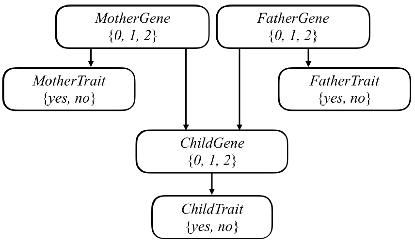
Each person in the family has a Gene random variable representing how many copies of a particular gene (e.g., the hearing impairment version of GJB2) a person has: a value that is 0, 1, or 2.
Each person in the family also has a Trait random variable, which is yes or no depending on whether that person expresses a trait (e.g., hearing impairment) based on that gene.
There’s an arrow from each person’s Gene variable to their Trait variable to encode the idea that a person’s genes affect the probability that they have a particular trait.
Meanwhile, there’s also an arrow from both the mother and father’s Gene random variable to their child’s Gene random variable: the child’s genes are dependent on the genes of their parents.
The task in this problem is to use this model to make inferences about a population. Given information about people, who their parents are, and whether they have a particular observable trait (e.g. hearing loss) caused by a given gene, the AI agent will infer the probability distribution for each person’s genes, as well as the probability distribution for whether any person will exhibit the trait in question.
The next figure shows the concepts required for running inference on a Bayes Network

Recall that to compute a joint probability of multiple events, you can do so by multiplying those probabilities together. But remember that for any child, the probability of them having a certain number of genes is conditional on what genes their parents have.
The following figure shows the given data files
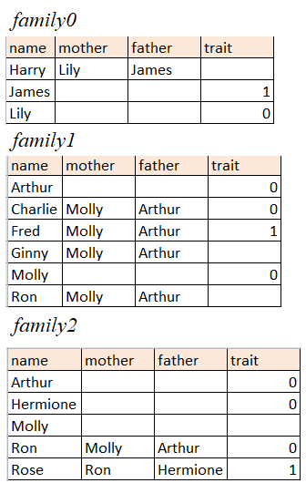
Implement a function joint_probability() that should take as input a dictionary of people, along with data about who has how many copies of each of the genes, and who exhibits the trait. The function should return the joint probability of all of those events taking place.
Implement a function update() that adds a new joint distribution probability to the existing probability distributions in probabilities .
Implement the function normalize() that updates a dictionary of probabilities such that each probability distribution is normalized.
PROBS is a dictionary containing a number of constants representing probabilities of various different events. All of these events have to do with how many copies of a particular gene a person has , and whether a person exhibits a particular trait based on that gene.
PROBS[“gene”] represents the unconditional probability distribution over the gene (i.e., the probability if we know nothing about that person’s parents).
PROBS[“trait”] represents the conditional probability that a person exhibits a trait.
PROBS[“mutation”] is the probability that a gene mutates from being the gene in question to not being that gene, and vice versa.
The following python code snippet shows how to compute the joint probabilities:
def joint_probability(people, one_gene, two_genes, have_trait):
"""
Compute and return a joint probability.
The probability returned should be the probability that
* everyone in set `one_gene` has one copy of the gene, and
* everyone in set `two_genes` has two copies of the gene, and
* everyone not in `one_gene` / `two_gene` doesn't have the gene
* everyone in set `have_trait` has the trait, and
* everyone not in set` have_trait` does not have the trait.
"""
prob_gene = PROBS['gene']
prob_trait_gene = PROBS['trait']
prob_mutation = PROBS['mutation']
prob_gene_pgenes = { # CPT
2: {
0: {
0: (1-prob_mutation)*prob_mutation,
1: (1-prob_mutation)*(1-prob_mutation) + \
prob_mutation*prob_mutation,
2: prob_mutation*(1-prob_mutation)
},
1: {
0: prob_mutation/2,
1: 0.5,
2: (1-prob_mutation)/2
},
2: {
0: prob_mutation*prob_mutation,
1: 2*(1-prob_mutation)*prob_mutation,
2: (1-prob_mutation)*(1-prob_mutation)
}
},
# compute the probabilities for the other cases...
}
all_probs = {}
for name in people:
has_trait = name in have_trait
num_gene = 1 if name in one_gene else 2 if name in two_genes
else 0
prob = prob_trait_gene[num_gene][has_trait]* \
prob_gene[num_gene]
if people[name]['mother'] != None:
mother, father = people[name]['mother'], \
people[name]['father']
num_gene_mother = 1 if mother in one_gene else \
2 if mother in two_genes else 0
num_gene_father = 1 if father in one_gene else 2
if father in two_genes else 0
prob = prob_trait_gene[num_gene][has_trait] * \
prob_gene_pgenes[num_gene_mother][num_gene_father] \
[num_gene]
all_probs[name] = prob
probability = np.prod(list(all_probs.values()))
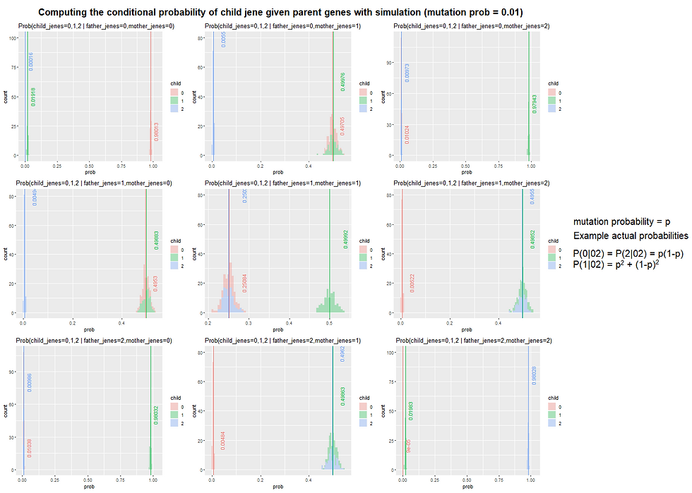
return probabilityThe following animations show how the CPTs (conditional probability tables) are computed for the Bayesian Networks corresponding to the three families, respectively.
The following figure shows the conditional probabilities (computed with simulation) that children does / doesn’t have the gene given the parents does / doesn’t have the gene.
Crossword
Write an AI agent to generate crossword puzzles.
Given the structure of a crossword puzzle (i.e., which squares of the grid are meant to be filled in with a letter), and a list of words to use, the problem becomes one of choosing which words should go in each vertical or horizontal sequence of squares.
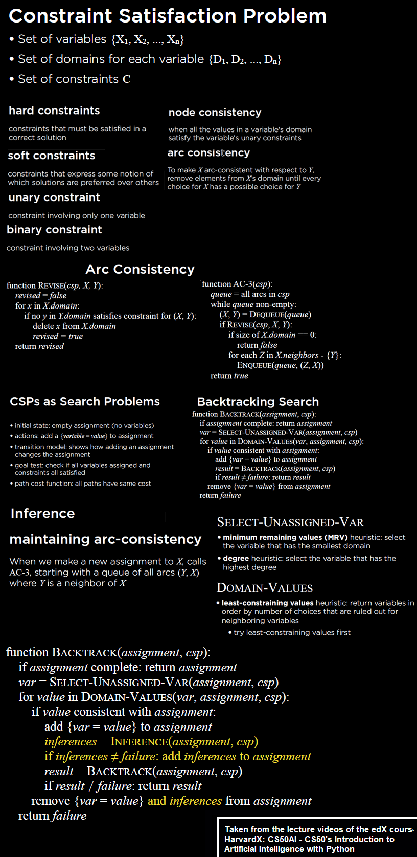
We can model this sort of problem as a constraint satisfaction problem.
Each sequence of squares is one variable, for which we need to decide on its value(which word in the domain of possible words will ll in that sequence). Consider the following crossword puzzle structure.
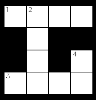
In this structure, we have four variables, representing the four words we need to ll into this crossword puzzle (each indicated by a number in the above image). Each variable is defined by four values: the row it begins on (its i value), the column it begins on (its j value), the direction of the word (either down or across), and the length of the word.
Variable 1, for example, would be a variable represented by a row of 1 (assuming 0 indexed counting from the top), a column of 1 (also assuming 0 indexed counting from the left), a direction of across, and a length of 4.
As with many constraint satisfaction problems, these variables have both unary and binary constraints. The unary constraint on a variable is given by its length.
For Variable 1, for instance, the value BYTE would satisfy the unary constraint, but the value BIT would not (it has the wrong number of letters).
Any values that don’t satisfy a variable’s unary constraints can therefore be removed from the variable’s domain immediately.
The binary constraints on a variable are given by its overlap with neighboring variables. Variable 1 has a single neighbor: Variable 2. Variable 2 has two neighbors: Variable 1 and Variable 3.
For each pair of neighboring variables, those variables share an overlap: a single square that is common to them both.
We can represent that overlap as the character index in each variable’s word that must be the same character.
For example, the overlap between Variable 1 and Variable 2 might be represented as the pair (1, 0), meaning that Variable 1’s character at index 1 necessarily must be the same as Variable 2’s character at index 0 (assuming 0-indexing, again).
The overlap between Variable 2 and Variable 3 would therefore be represented as the pair (3, 1): character 3 of Variable 2’s value must be the same as character 1 of Variable 3’s value.
For this problem, we’ll add the additional constraint that all words must be different: the same word should not be repeated multiple times in the puzzle.
The challenge ahead, then, is write a program to find a satisfying assignment: a different word (from a given vocabulary list) for each variable such that all of the unary and binary constraints are met.
The following figure shows the theory required to solve the problem:
Implement a function enforce_node_consistency() that should update the domains such that each variable is node consistent.
Implement a function ac3() that should, using the AC3 algorithm, enforce arc consistency on the problem. Recall that arc consistency is achieved when all the values in each variable’s domain satisfy that variable’s binary constraints.
Recall that the AC3 algorithm maintains a queue of arcs to process. This function takes an optional argument called arcs, representing an initial list of arcs to process. If arcs is None, the function should start with an initial queue of all of the arcs in the problem. Otherwise, the algorithm should begin with an initial queue of only the arcs that are in the list arcs.
Implement a function consistent() that should check to see if a given assignment is consistent and a function assignment_complete() that should check if a given assignment is complete.
Implement a function select_unassigned_variable() that should return a single variable in the crossword puzzle that is not yet assigned by assignment, according to the minimum remaining value heuristic and then the degree heuristic. Also, it should return the variable with the fewest number of remaining values in its domain.
Implement a function backtrack() that should accept a partial assignment as input and, using backtracking search, return a complete satisfactory assignment of variables to values if it is possible to do so.
The following python code snippet shows couple of the above function implementations:
def select_unassigned_variable(self, assignment):
    """
    Return an unassigned variable not already part of `assignment`.
    Choose the variable with the minimum number of remaining values
    in its domain. If there is a tie, choose the variable with the
    highest degree. If there is a tie, any of the tied variables
    are acceptable return values.
    """
    unassigned_vars = list(self.crossword.variables - \
                               set(assignment.keys()))
    mrv, svar = float('inf'), None
    for var in unassigned_vars:
        if len(self.domains[var]) < mrv:
           mrv, svar =  len(self.domains[var]), var
        elif len(self.domains[var]) == mrv:
           if self.crossword.neighbors(var) >
              self.crossword.neighbors(svar):
              svar = var
    return svar

def backtrack(self, assignment):
    """
    Using Backtracking Search, take as input a partial assignment
    for the crossword and return a complete assignment if possible
    to do so.
    `assignment` is a mapping from variables (keys) to words
    (values).
    If no assignment is possible, return None.
    """
    # Check if assignment is complete
    if len(assignment) == len(self.crossword.variables):
    return assignment    # Try a new variable
    var = self.select_unassigned_variable(assignment)
    for value in self.domains[var]:
        new_assignment = assignment.copy()
        new_assignment[var] = value
        if self.consistent(new_assignment):
           result = self.backtrack(new_assignment)
           if result is not None:
              return result
    return None
The following animation shows how the backtracking algorithm with AC3 generates the crossword with the given structure.
######_
____##_
_##____
_##_##_
_##_##_
#___##_
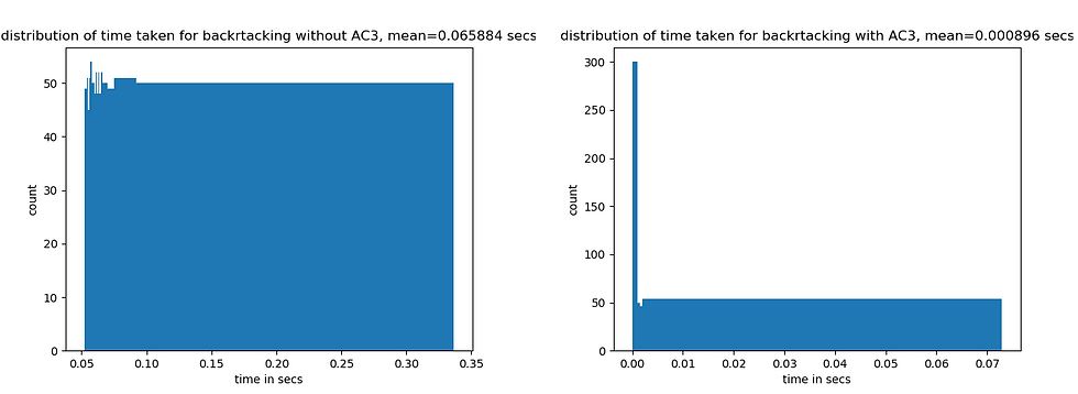
Now let’s compute the speedup obtained with backtracking with and without AC3 (on average), i.e., compare the time to generate a crossword puzzle (with the above structure), averaged over 1000 runs (each time the puzzle generated may be different though). The next figure shows the result of the runtime experiment and that backtracking with AC3 is way faster on average over backtracking implementation without AC3.
Shopping
Write an AI agent to predict whether online shopping customers will complete a purchase.
When users are shopping online, not all will end up purchasing something. Most visitors to an online shopping website, in fact, likely don’t end up going through with a purchase during that web browsing session.
It might be useful, though, for a shopping website to be able to predict whether a user intends to make a purchase or not: perhaps displaying different content to the user, like showing the user a discount offer if the website believes the user isn’t planning to complete the purchase.
How could a website determine a user’s purchasing intent? That’s where machine learning will come in.
The task in this problem is to build a nearest-neighbor classifier to solve this problem. Given information about a user — how many pages they’ve visited, whether they’re shopping on a weekend, what web browser they’re using, etc. — the classifier will predict whether or not the user will make a purchase.
The classifier won’t be perfectly accurate — but it should be better than guessing randomly.
To train the classifier a dataset from a shopping website from about 12,000 users sessions is provided.
How do we measure the accuracy of a system like this? If we have a testing data set, we could run our classifier and compute what proportion of the time we correctly classify the user’s intent.
This would give us a single accuracy percentage. But that number might be a little misleading. Imagine, for example, if about 15% of all users end up going through with a purchase. A classifier that always predicted that the user would not go through with a purchase, then, we would measure as being 85% accurate: the only users it classifies incorrectly are the 15% of users who do go through with a purchase. And while 85% accuracy sounds pretty good, that doesn’t seem like a very useful classifier.
Instead, we’ll measure two values: sensitivity (also known as the “true positive rate”) and specificity (also known as the “true negative rate”).
Sensitivity refers to the proportion of positive examples that were correctly identified: in other words, the proportion of users who did go through with a purchase who were correctly identified.
Specificity refers to the proportion of negative examples that were correctly identified: in this case, the proportion of users who did not go through with a purchase who were correctly identified.
So our “always guess no” classifier from before would have perfect specificity (1.0) but no sensitivity (0.0). Our goal is to build a classifier that performs reasonably on both metrics.
First few rows from the csv dataset are shown in the following figure:

There are about 12,000 user sessions represented in this spreadsheet: represented as one row for each user session.
The first six columns measure the different types of pages users have visited in the session: the Administrative , Informational , and ProductRelated columns measure how many of those types of pages the user visited, and their corresponding _Duration columns measure how much time the user spent on any of those pages.
The BounceRates , ExitRates , and PageValues columns measure information from Google Analytics about the page the user visited. SpecialDay is a value that measures how closer the date of the user’s session is to a special day (like Valentine’s Day or Mother’s Day).
Month is an abbreviation of the month the user visited. OperatingSystems , Browser , Region, and TrafficType are all integers describing information about the user themself.
VisitorType will take on the value Returning_Visitor for returning visitors and New_Visitor for new visitors to the site.
Weekend is TRUE or FALSE depending on whether or not the user is visiting on a weekend.
Perhaps the most important column, though, is the last one: the Revenue column. This is the column that indicates whether the user ultimately made a purchase or not: TRUE if they did, FALSE if they didn’t. This is the column that we’d like to learn to predict (the “label”), based on the values for all of the other columns (the “evidence”).
Implement a function load_data() that should accept a CSV filename as its argument, open that file, and return a tuple (evidence, labels) . evidence should be a list of all of the evidence for each of the data points, and labels should be a list of all of the labels for each data point.
Implement a function train_model() function should accept a list of evidence and a list of labels, and return a scikit-learn nearest-neighbor classifier (a k-nearest-neighbor classifier where k = 1) fitted on that training data.
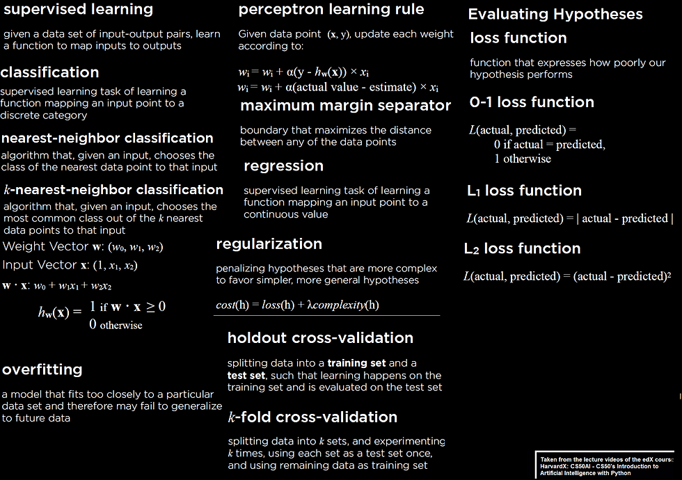
Relevant concepts in supervised machine learning (classification) needed for this problem is described in the following figure.
Use the following python code snippet to divide the dataset into two parts: the first one to train the 1-NN model on and the second one being a held-out test dataset to evaluate the model using the performance metrics.
from sklearn.model_selection import train_test_split
from sklearn.neighbors import KNeighborsClassifier
TEST_SIZE = 0.4# Load data from spreadsheet and split into train and test sets
evidence, labels = load_data('shopping.csv')
X_train, X_test, y_train, y_test = train_test_split(
   evidence, labels, test_size=TEST_SIZE
)
# Train model and make predictions
model = train_model(X_train, y_train)
predictions = model.predict(X_test)
sensitivity, specificity = evaluate(y_test, predictions)def train_model(evidence, labels):
    """
    Given a list of evidence lists and a list of labels, return a
    fitted k-nearest neighbor model (k=1) trained on the data.
    """
    model = KNeighborsClassifier(n_neighbors=1)
    model.fit(evidence, labels)
    return model
With 60–40 validation with a sample run following result is obtained, by training the model on 60% training data and use the model to predict on the 40% held-out test dataset, and then comparing the test predictions with the ground truth:
Correct: 3881
Incorrect: 1051
True Positive Rate: 31.14%
True Negative Rate: 87.37%
Now, let’s repeat the experiment for 25 times (with different random seeds for train_test_split()) and let’s plot the sensitivity against specificity for every random partition, along with color-coded accuracy, to obtain a plot like the following one.
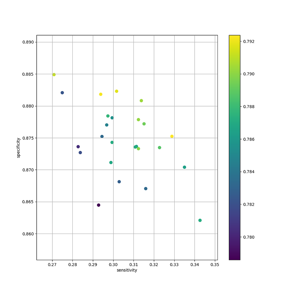
with the mean performance metrics reported as follows (to reduce the variability in the result):
Sensitivity: 0.3044799546457174
Specificity: 0.8747533289505658
Accuracy: 0.7867234387672343
As can be seen from the above result, the specificity if quite good, but sensitivity obtained is quite poor.
Let’s now plot the decision boundary obtained with 1-NN classifier for different 60–40 train-test validation datasets created, with the data projected across two principal components, the output is shown in the following animation (here the red points represent the cases where purchase happened and the blue points represent the cases where it did not).
Nim
Implement an AI agent that teaches itself to play Nim through reinforcement learning.
Recall that in the game Nim, we begin with some number of piles, each with some number of objects. Players take turns: on a player’s turn, the player removes any non-negative number of objects from any one non-empty pile. Whoever removes the last object loses.
There’s some simple strategy you might imagine for this game: if there’s only one pile and three objects left in it, and it’s your turn, your best bet is to remove two of those objects, leaving your opponent with the third and final object to remove.
But if there are more piles, the strategy gets considerably more complicated. In this problem, we’ll build an AI agent to learn the strategy for this game through reinforcement learning. By playing against itself repeatedly and learning from experience, eventually our AI agent will learn which actions to take and which actions to avoid.
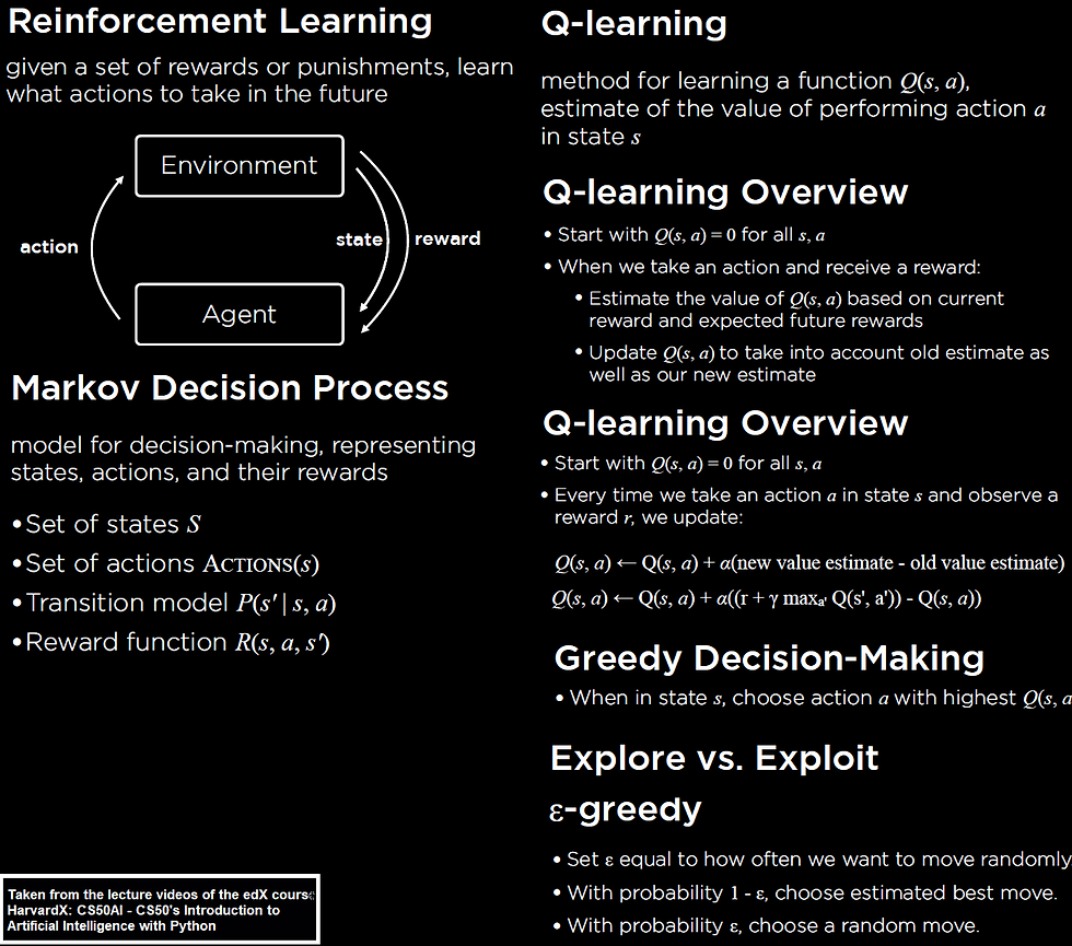
In particular, we’ll use Q-learning for this project. Recall that in Q-learning, we try to learn a reward value (a number) for every (state,action) pair. An action that loses the game will have a reward of -1, an action that results in the other player losing the game will have a reward of 1, and an action that results in the game continuing has an immediate reward of 0, but will also have some future reward.
How will we represent the states and actions inside of a Python program? A “state” of the Nim game is just the current size of all of the piles. A state, for example, might be [1, 1, 3, 5] , representing the state with 1 object in pile 0, 1 object in pile 1, 3 objects in pile 2, and 5 objects in pile 3. An “action” in the Nim game will be a pair of integers (i, j) , representing the action of taking j objects from pile i . So the action (3, 5) represents the action “from pile 3, take away 5 objects.” Applying that action to the state [1, 1, 3, 5] would result in the new state [1, 1, 3, 0] (the same state, but with pile 3 now empty).
Recall that the key formula for Q-learning is below. Every time we are in a state s and take an action a , we can update the Q-value Q(s, a) according to: Q(s, a) <- Q(s, a) + alpha * (new value estimate — old value estimate)
In the above formula, alpha is the learning rate (how much we value new information compared to information we already have).
The new value estimate represents the sum of the reward received for the current action and the estimate of all the future rewards that the player will receive.
The old value estimate is just the existing value for Q(s, a) . By applying this formula every time our AI agent takes a new action, over time our AI agent will start to learn which actions are better in any state.
The concepts required for reinforcement learning and Q-learning is shown in the following figure.
Next python code snippet shows how to implement q-values update for Q-learning with the update() method from the NimAI class.
class NimAI():    def update(self, old_state, action, new_state, reward):
        """
        Update Q-learning model, given an old state, an action taken
        in that state, a new resulting state, and the reward
        received from taking that action.
        """
        old = self.get_q_value(old_state, action)
        best_future = self.best_future_reward(new_state)
        self.update_q_value(old_state, action, old, reward,
                                                    best_future)    def update_q_value(self, state, action, old_q, reward,
                                                   future_rewards):
        """
        Update the Q-value for the state `state` and the action
        `action` given the previous Q-value `old_q`, a current
        reward `reward`, and an estimate of future rewards
        `future_rewards`.
        Use the formula:        Q(s, a) <- old value estimate
                 + alpha * (new value estimate - old value estimate)        where `old value estimate` is the previous Q-value,
        `alpha` is the learning rate, and `new value estimate`
        is the sum of the current reward and estimated future
        rewards.
        """
        self.q[(tuple(state), action)] = old_q + self.alpha * (
                              (reward + future_rewards) - old_q)
The AI agent plays 10000 training games to update the q-values, the following animation shows how the q-values are updated in last few games (corresponding to a few selected states and action pairs):
The following animation shows an example game played between the AI agent (the computer) and the human (the green, red and white boxes in each row of the first subplot represent the non-empty, to be removed and empty piles for the corresponding row, respectively, for the AI agent and the human player).

As can be seen from the above figure, one of actions with the highest q-value for the AI agent’s first turn is (3,6) , that’s why it removes 6 piles from the 3rd row. Similarly, in the second tun of the AI agent, one of the best actions is (2,5), that’s why it removes 5 piles from row 2 and likewise.
The following animation shows another example game AI agent plays with human:
Traffic
Write an AI agent to identify which traffic sign appears in a photograph.
As research continues in the development of self-driving cars, one of the key challenges is computer vision, allowing these cars to develop an understanding of their environment from digital images.
In particular, this involves the ability to recognize and distinguish road signs — stop signs, speed limit signs, yield signs, and more.
The following figure contains the theory required to perform the multi-class classification task using a deep neural network.

In this problem, we shall use TensorFlow (https://www.tensorow.org/) to build a neural network to classify road signs based on an image of those signs.
To do so, we shall need a labeled dataset: a collection of images that have already been categorized by the road sign represented in them.
Several such data sets exist, but for this project, we’ll use the German Traffic Sign Recognition Benchmark (http://benchmark.ini.rub.de/?section=gtsrb&subsection=news) (GTSRB) dataset, which contains thousands of images of 43 different kinds of road signs.
The dataset contains 43 sub-directories, numbered 0 through 42. Each numbered sub-directory represents a different category (a different type of road sign). Within each traffic sign’s directory is a collection of images of that type of traffic sign.
Implement the load_data() function which should accept as an argument data_dir, representing the path to a directory where the data is stored, and return image arrays and labels for each image in the data set.
While loading the dataset, the images have to be resized to a fixed size. If the images are resized correctly, each of them will have shape as (30, 30, 3).
Also, implement the function get_model() which should return a compiled neural network model.
The following python code snippet shows how to implement the classification model with keras, along with the output produced when the model is run.
import numpy as np
import tensorflow as tfEPOCHS = 10
IMG_WIDTH = 30
IMG_HEIGHT = 30
NUM_CATEGORIES = 43
TEST_SIZE = 0.4# Get image arrays and labels for all image files
images, labels = load_data('gtsrb')# Split data into training and testing sets
labels = tf.keras.utils.to_categorical(labels)
x_train, x_test, y_train, y_test = train_test_split(
np.array(images), np.array(labels), test_size=TEST_SIZE
)# Get a compiled neural network
model = get_model()# Fit model on training data
model.fit(x_train, y_train, epochs=EPOCHS)# Evaluate neural network performance
model.evaluate(x_test, y_test, verbose=2)def get_model():
"""
Returns a compiled convolutional neural network model.
Assume that the `input_shape` of the first layer is
`(IMG_WIDTH, IMG_HEIGHT, 3)`.
The output layer should have `NUM_CATEGORIES` units, one for
each category.
"""
# Create a convolutional neural network
model = tf.keras.models.Sequential([
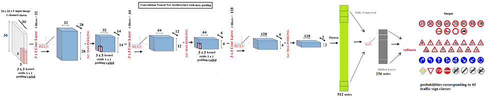
# Convolutional layer. Learn 32 filters using a 3x3 kernel
tf.keras.layers.Conv2D(
32, (3, 3), activation="relu", input_shape=(30, 30, 3)
),
# Max-pooling layer, using 2x2 pool size
tf.keras.layers.MaxPooling2D(pool_size=(2, 2)),
# Convolutional layer. Learn 32 filters using a 3x3 kernel
tf.keras.layers.Conv2D(
64, (3, 3), activation="relu"
),
# Max-pooling layer, using 2x2 pool size
tf.keras.layers.MaxPooling2D(pool_size=(2, 2)),
tf.keras.layers.Conv2D(
128, (3, 3), activation="relu"
),
# Max-pooling layer, using 2x2 pool size
tf.keras.layers.MaxPooling2D(pool_size=(2, 2)),
# Flatten units
tf.keras.layers.Flatten(),
# Add a hidden layer with dropout
tf.keras.layers.Dense(256, activation="relu"),
tf.keras.layers.Dropout(0.5),
# Add an output layer with output units for all 10 digits
tf.keras.layers.Dense(NUM_CATEGORIES, activation="softmax")
])
print(model.summary) # Train neural network
model.compile(
optimizer="adam",
loss="categorical_crossentropy",
metrics=["accuracy"]
)
return model
# Model: "sequential"
# _________________________________________________________________
# Layer (type) Output Shape Param #
# =================================================================
# conv2d (Conv2D) (None, 28, 28, 32) 896
# _________________________________________________________________
# max_pooling2d (MaxPooling2D) (None, 14, 14, 32) 0
# _________________________________________________________________
# conv2d_1 (Conv2D) (None, 12, 12, 64) 18496
# _________________________________________________________________
# max_pooling2d_1 (MaxPooling2 (None, 6, 6, 64) 0
# _________________________________________________________________
# conv2d_2 (Conv2D) (None, 4, 4, 128) 73856
# _________________________________________________________________
# max_pooling2d_2 (MaxPooling2 (None, 2, 2, 128) 0
# _________________________________________________________________
# flatten (Flatten) (None, 512) 0
# _________________________________________________________________
# dense (Dense) (None, 256) 131328
# _________________________________________________________________
# dropout (Dropout) (None, 256) 0
# _________________________________________________________________
# dense_1 (Dense) (None, 43) 11051
# =================================================================
# Total params: 235,627
# Trainable params: 235,627
# Non-trainable params: 0
# _________________________________________________________________The architecture of the deep network is shown in the next figure:
The following output shows how the cross-entropy loss on the training dataset decreases and the accuracy of classification increases over epochs on the training dataset.
Epoch 1/10
15864/15864 [==============================] - 17s 1ms/sample - loss: 2.3697 - acc: 0.4399
Epoch 2/10
15864/15864 [==============================] - 15s 972us/sample - loss: 0.6557 - acc: 0.8133
Epoch 3/10
15864/15864 [==============================] - 16s 1ms/sample - loss: 0.3390 - acc: 0.9038
Epoch 4/10
15864/15864 [==============================] - 16s 995us/sample - loss: 0.2526 - acc: 0.9285
Epoch 5/10
15864/15864 [==============================] - 16s 1ms/sample - loss: 0.1992 - acc: 0.9440
Epoch 6/10
15864/15864 [==============================] - 16s 985us/sample - loss: 0.1705 - acc: 0.9512
Epoch 7/10
15864/15864 [==============================] - 15s 956us/sample - loss: 0.1748 - acc: 0.9536
Epoch 8/10
15864/15864 [==============================] - 15s 957us/sample - loss: 0.1551 - acc: 0.9578
Epoch 9/10
15864/15864 [==============================] - 16s 988us/sample - loss: 0.1410 - acc: 0.9630
Epoch 10/10
15864/15864 [==============================] - 14s 878us/sample - loss: 0.1303 - acc: 0.9667
10577/10577 - 3s - loss: 0.1214 - acc: 0.9707
The following animation again shows how the cross-entropy loss on the training dataset decreases and the accuracy of classification increases over epochs on the training dataset.
The following figure shows a few sample images from the traffic dataset with different labels.

The next animations show the features learnt at various convolution and pooling layers.
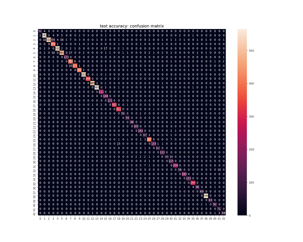
The next figure shows the evaluation result on test dataset — the corresponding confusion matrix.
Parser
Write an AI agent to parse sentences and extract noun phrases.
A common task in natural language processing is parsing, the process of determining the structure of a sentence.
This is useful for a number of reasons: knowing the structure of a sentence can help a computer to better understand the meaning of the sentence, and it can also help the computer extract information out of a sentence.
In particular, it’s often useful to extract noun phrases out of a sentence to get an understanding for what the sentence is about.
In this problem, we’ll use the context-free grammar formalism to parse English sentences to determine their structure.
Recall that in a context-free grammar, we repeatedly apply rewriting rules to transform symbols into other symbols. The objective is to start with a non-terminal symbol S (representing a sentence) and repeatedly apply context-free grammar rules until we generate a complete sentence of terminal symbols (i.e., words).
The rule S -> N V , for example, means that the S symbol can be rewritten as N V (a noun followed by a verb). If we also have the rule N -> “Holmes” and the rule V -> “sat” , we can generate the complete sentence “Holmes sat.” .
Of course, noun phrases might not always be as simple as a single word like “Holmes” . We might have noun phrases like “my companion” or “a country walk” or “the day before Thursday” , which require more complex rules to account for.
To account for the phrase “my companion” , for example, we might imagine a rule like: NP -> N | Det N. In this rule, we say that an NP (a “noun phrase”) could be either just a noun ( N ) or a determiner ( Det ) followed by a noun, where determiners include words like “a” , “the” , and “my” . The vertical bar ( | ) just indicates that there are multiple possible ways to rewrite an NP , with each possible rewrite separated by a bar.
To incorporate this rule into how we parse a sentence ( S ), we’ll also need to modify our S -> N V rule to allow for noun phrases ( NP s) as the subject of our sentence. See how? And to account for more complex types of noun phrases, we may need to modify our grammar even further.
Given sentences that are needed to be parsed by the CFG (to be constructed) are shown below:
Holmes sat.
Holmes lit a pipe.
We arrived the day before Thursday.
Holmes sat in the red armchair and he chuckled.
My companion smiled an enigmatical smile.
Holmes chuckled to himself.
She never said a word until we were at the door here.
Holmes sat down and lit his pipe.
I had a country walk on Thursday and came home in a dreadful mess.
I had a little moist red paint in the palm of my hand.
Implementation tips
The NONTERMINALS global variable should be replaced with a set of context-free grammar rules that, when combined with the rules in TERMINALS , allow the parsing of all sentences in the sentences/ directory.
Each rules must be on its own line. Each rule must include the -> characters to denote which symbol is being replaced, and may optionally include | symbols if there are multiple ways to rewrite a symbol.
Do not need to keep the existing rule S -> N V in your solution, but the first rule must begin with S -> since S (representing a sentence) is the starting symbol.
May add as many nonterminal symbols as needed.
Use the nonterminal symbol NP to represent a “noun phrase”, such as the subject of a sentence.
A few rules needed to parse the given sentences are shown below (we need to add a few more rules):
NONTERMINALS = """
S -> NP VP | S Conj VP | S Conj S | S P S
NP -> N | Det N | AP NP | Det AP NP | N PP | Det N PP
"""
Few rules for the TERMINALS from the given grammar are shown below:
TERMINALS = """
Adj -> "country" | "dreadful" | "enigmatical" | "little" | "moist" | "red"
Conj -> "and"
Det -> "a" | "an" | "his" | "my" | "the"
N -> "armchair" | "companion" | "day" | "door" | "hand" | "he" | "himself"
P -> "at" | "before" | "in" | "of" | "on" | "to" | "until"
V -> "smiled" | "tell" | "were"
"""
The next python code snippet implements the function np_chunk() that should accept a nltk tree representing the syntax of a sentence, and return a list of all of the noun phrase chunks in that sentence.
For this problem, a “noun phrase chunk” is defined as a noun phrase that doesn’t contain other noun phrases within it. Put more formally, a noun phrase chunk is a subtree of the original tree whose label is NP and that does not itself contain other noun phrases as subtrees.
Assume that the input will be a nltk.tree object whose label is S (that is to say, the input will be a tree representing a sentence).
The function should return a list of nltk.tree objects, where each element has the label NP.
The documentation for nltk.tree will be helpful for identifying how to manipulate a nltk.tree object.
import nltkdef np_chunk(tree):
    """
    Return a list of all noun phrase chunks in the sentence tree.
    A noun phrase chunk is defined as any subtree of the sentence
    whose label is "NP" that does not itself contain any other
    noun phrases as subtrees.
    """
    chunks = []
    for s in tree.subtrees(lambda t: t.label() == 'NP'):
       if len(list(s.subtrees(lambda t: t.label() == 'NP' and
                                        t != s))) == 0:
        chunks.append(s)
    return chunks
The following animation shows how the given sentences are parsed with the grammar rules constructed.
Questions
Write an AI agent to answer questions from a given corpus
Question Answering (QA) is a field within natural language processing focused on designing systems that can answer questions.
Among the more famous question answering systems is Watson , the IBM computer that competed (and won) on Jeopardy!.
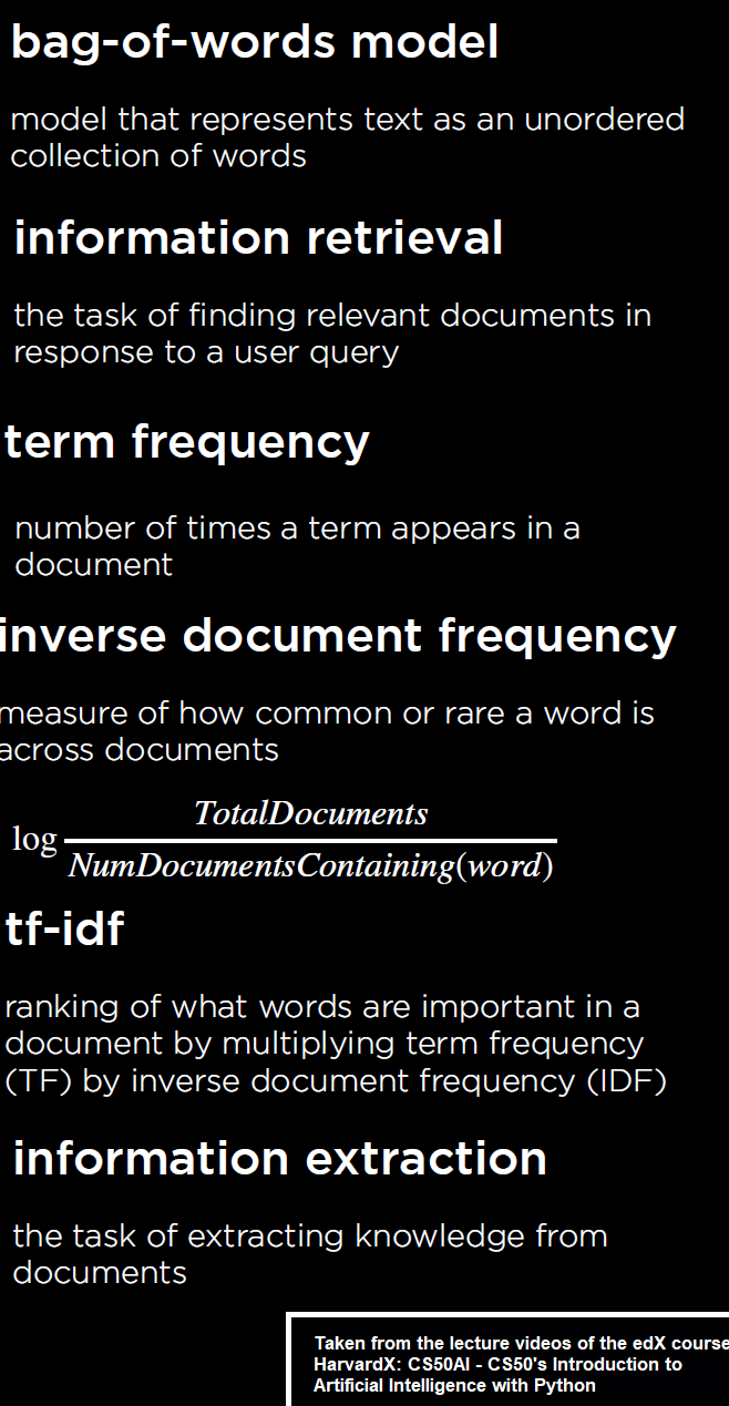
A question answering system of Watson’s accuracy requires enormous complexity and vast amounts of data, but in this problem, we’ll design a very simple question answering system based on inverse document frequency.
Our question answering system will perform two tasks: document retrieval and passage retrieval.
Our system will have access to a corpus of text documents.
When presented with a query (a question in English asked by the user), document retrieval will first identify which document(s) are most relevant to the query.
Once the top documents are found, the top document(s) will be subdivided into passages (in this case, sentences) so that the most relevant passage to the question can be determined.
How do we find the most relevant documents and passages? To find the most relevant documents, we’ll use tf-idf to rank documents based both on term frequency for words in the query as well as inverse document frequency for words in the query. The required concepts are summarized in the following figure:
Once we’ve found the most relevant documents, there are many possible metrics for scoring passages, but we’ll use a combination of inverse document frequency and a query term density measure.
More sophisticated question answering systems might employ other strategies (analyzing the type of question word used, looking for synonyms of query words, lemmatizing to handle different forms of the same word, etc.), but that comes only after the baseline version is implemented.
Implementation tips
Implement a function compute_idfs() that should accept a dictionary of documents and return a new dictionary mapping words to their IDF (inverse document frequency) values.
Assume that documents will be a dictionary mapping names of documents to a list of words in that document.
The returned dictionary should map every word that appears in at least one of the documents to its inverse document frequency value.
Recall that the inverse document frequency of a word is defined by taking the natural logarithm of the number of documents divided by the number of documents in which the word appears.
Implement the top_files() function that should, given a query (a set of words), files (a dictionary mapping names of files to a list of their words), and idfs (a dictionary mapping words to their IDF values), return a list of the filenames the n top files that that match the query, ranked according to tf-idf.
The returned list of should be of length n and should be ordered with the best match first.
Files should be ranked according to the sum of tf-idf values for any word in the query that also appears in the file. Words in the query that do not appear in the file should not contribute to the file’s score.
Recall that tf-idf for a term is computed by multiplying the number of times the term appears in the document by the IDF value for that term.
Implement the function top_sentences() that should, given a query (a set of words), sentences (a dictionary mapping sentences to a list of their words), and idfs (a dictionary mapping words to their IDF values), return a list of the n top sentences that match the query, ranked according to IDF.
The returned list of sentences should be of length n and should be ordered with the best match first.
Sentences should be ranked according to “matching word measure”: namely, the sum of IDF values for any word in the query that also appears in the sentence. Note that term frequency should not be taken into account here, only inverse document frequency.
If two sentences have the same value according to the matching word measure, then sentences with a higher “query term density” should be preferred. Query term density is defined as the proportion of words in the sentence that are also words in the query.
The next python code snippet shows how the couple of functions mentioned above are implemented:
def compute_idfs(documents):
    """
    Given a dictionary of `documents` that maps names of documents
    to a list of words, return a dictionary that maps words to their
    IDF values.
    Any word that appears in at least one of the documents should
    be in the resulting dictionary.
    """
    words = set()
    for document in documents:
        words.update(documents[document])
    idfs = dict()
    for word in words:
        f = sum(word in documents[document] for document in
                                                documents)
        idfs[word] = math.log(len(documents) / f)
    return idfsdef top_files(query, files, idfs, n):
    """
    Given a `query` (a set of words), `files` (a dictionary mapping
    names of files to a list of their words), and `idfs` (a
    dictionary mapping words to their IDF values), return a list of
    the filenames of the the `n` top files that match the query,
    ranked according to tf-idf.
    """
    scores = []
    for filename in files:
        score = 0
        for word in query:
            tf = len(list(filter(lambda w: w == word,
                                           files[filename])))
            score += tf * idfs.get(word, 0)
        scores.append((score, filename))
    scores.sort(key = lambda x: -x[0])
    return [item[1] for item in scores][:n]
The following animation shows the answers to the questions found from the given corpus: for each question, the best candidate text (document) likely containing the answer is first found inside the corpus and then the top 5 candidate answer sentences is found inside that document.
Artificial Intelligence is a vast area of research and it contains many different sub-areas those themselves are huge. In this blog, we discussed some problems from Search, Knowledge (Logic) and Uncertainty, Optimization, Learning, Neural Network and Language. We discussed how to implement AI agents for an adversarial search game (tic-tac-toe), a logic-based game (minesweeper) and a reinforcement learning-based game (Nim). We have also seen how to generate crossword puzzles by representing the problem as a CSP problem. Finally, we have seen application of AI in Computer Vision (traffic sign classification needed for self driving cars) and NLP (question-answering system with information retrieval).


Comments